Download

1 / 17
170 likes | 325 Views
L-THIA in ArcGIS L-THIA in Python project. July 2010 Larry Theller theller@purdue.edu. Notes. Current python script to read netCDF should change to convert mm into inches; and the output value should be inch times 100, Output is integer. Test full size 3 geotif rasters:

E N D
L-THIA in ArcGIS L-THIA in Python project July 2010 Larry Theller theller@purdue.edu
Notes • Current python script to read netCDF should change to convert mm into inches; and the output value should be inch times 100, • Output is integer. • Test full size 3 geotif rasters: • CN_grid.tif, precip_code.tif , results.tif • Test small size geotif rasters: • p256.tif and p257.tif these are CN maps of future precip pixels 256 and 257
Basics • NetCDf precipitation file in mm • Pixel is 6 or 8 KM2 • NetCDF is 366 bands of data in an archive with metadata embedded • Standard GIS software only reads 200 bands • Need to “decode” netCDF somehow (.net, python, etc.)
Zoom in to precipitation pixel One Precipitation pixel is 6 to 8 KM square
“Curve Number” map One CN pixel is 30 by 30 m
Calculation • Predicting Runoff Volume by Curve Number: • Water conveyance measures are sized by peak runoff rates. Water supply systems for irrigation or other water consumptive use are sized on the basis of runoff volume. The Natural Resources Conservation Service* Curve Number Method can predict a complete runoff hydrograph, but it will not be so used in this course. It predicts runoff volume, Q, by the formula: • where: • Q = direct runoff volume, in. I = storm rainfall depth, in. (ave. intensity x duration) [ or use avg daily precipitation ]S = (1000/CN) - 10 CN = runoff curve number • Curve number is based on the soils and land uses in the watershed (see CN-table). • For single calculation representing a watershed, in nonuniform watersheds an area-weighted average is used. Rainfall depth, I, is estimated for a given recurrence interval and duration for the location in question. (in this project 24 hrs.)
Look-up table Rather than calculate 340 million times we propose to read precip value, CN value and do a look –up over and over. CN is one dimension and precip is the other, all possible answers are precalculated. Repeat 365 times per year for each 30 by 30 meter pixel. This is storage then of 18,000 by 18,000 rows and columns – which is the problem.
netCDF project Simplified process: • Start with 3 exact Matching rasters of CN and precip_code and results ( results values all 0 at start) [ cn_grid.tif; precip_code.tif; results.tif ] • For each small pixel in CN, with GDAL (?) find same small pixel in precip-code which says what “big pixel” to use from the table or csv/array named PCRP1950.csv (made earler from netCDF with python) • For each small pixel in CN, do 366 days (or less) of look-ups, where big pixel precip values from netCDF table “PCRP1950.csv” and small pixel CN value are the 2 dimensions used ( CN column, precip rows) in table “lookup_mm_preci2_lu.csv “ which is precomputed runoff • sum these 366 lookups from lookup_mm_preci2_lu.csv into same small pixel in “results.tif”
I made a raster of the netcdf pixel number named precip_code.tif; this is exact same size and location small pixels as the CN_grid has. Has same origin and extent as the CN_grif.tif.
I made a raster for storing results named results.tif (I saw a GDAL operator to stick a value into a raster by column and row); this is exact same size and location small pixels as the CN_grid has. Has same origin and extent as the CN_grif.tif.
I got a python routine to make a csv file where each big pixel is a row and the 366 daily precip values are listed as columns. Row numbers match the values in raster precip_code.tif) So the CN small pixel value and the 366 values in the correct row (row = code number) are used in the lookup action against lookup_mm_preci2_lu.csv
Correct row highlighted. If this works we will want to continue through multiple years ( multiple of these files from netCDF)
So the CN pixel value and the 366 values in the correct row are used in the lookup action against this lookup_mm_preci2_lu.csv Then sum 366 lookups into array and finally into raster for storing results named results.tif (I saw a GDAL operator to stick a value into a raster by column and row); this is exact same size and location small pixels as the CN_grid has. Has same origin and extent as the CN_grid.tif.
I made two smaller subsets if you need them, p256.tif and p257.tif – to practice with if subset bookkeeping is needed. They are subset of wisconsin CN_grid.tif to match two “big pixel” areas.