Download
1 / 24
240 likes | 246 Views
Parameter Estimation. Chapter 8 Homework: 1-7, 9, 10 Focus: when s is known (use z table). Describing Populations. Chap 7 Knew population ---> describe samples Sampling distribution of means, standard error of the means Reality: usually do not know m , s impractical

E N D
Parameter Estimation Chapter 8 Homework: 1-7, 9, 10 Focus: when s is known (use z table)
Describing Populations • Chap 7 • Knew population ---> describe samples • Sampling distribution of means, standard error of the means • Reality: usually do not know m, s • impractical • Select representative sample • find statistics: X, s ~
Parameter Estimation • Know X ---> what is m ? • Estimation techniques • Point estimate • single value: X and s • Confidence interval • range of values • probably contains m ~
Point-estimation • X is an unbiased estimator • if repeated point-estimating infinitely... • as many X less than m as greater than • mode & median also unbiased estimator of m but neither is best estimator of m • X is best unbiased estimator of m~
Distribution Of Sample Means • How close is X to m? • look at sampling distribution of means • Probably within 2 standard errors of mean • about 96% of sample means • 2 standard errors above or below m • Probably: P=.95 (or .99, or .999, etc.) ~
P(X = m+ 2s) -2 -1 0 1 2 How close is X to m? »96% f
Distribution Of Sample Means • If area = .95 • exactly how many standard errors above/below m ? • Table A.1: proportions of area under normal curve • look up • .475: z = ~ 1.96
Critical Value of a Statistic • Value of statistic • that marks boundary of specified area • in tail of distribution • zCV.05= ±1.96 • area = .025 in each tail • 5% of X are beyond 1.96 • or 95% of X fall within 1.96 standard errors of mean ~
-2 -1 0 1 2 +1.96 -1.96 Critical Value of a Statistic f .95 .025 .025
Confidence Intervals • Range of values that m is expected to lie within • 95% confidence interval • .95 probability that mwill fall within range • probability is the level of confidence • e.g., .75 (uncommon), or .99 or .999 • Which level of confidence to use? • Cost vs. benefits judgement ~
< m < (s X) (s X) (s X) X - zCV X + zCV X ±zCV Lower limit Upper limit or Finding Confidence Intervals • Method depends on whether s is known • If s known
Meaning of Confidence Interval • 95% confident that m lies between lower & upper limit • NOT absolutely certain • .95 probability • If computed C.I. 100 times • using same methods • m within range about 95 times • Never know m for certain • 95% confident within interval ~
Example • Compute 95% C.I. • IQ scores • s = 15 • Sample: 114, 118, 122, 126 • SXi = 480, X = 120, sX = 7.5 • 120 ± 1.96(7.5) • 120 + 14.7 • 105.3 < m < 134.7 • We are 95% confident that population means lies between 105.3 and 134.7 ~
Changing the Level of Confidence • We want to be 99% confident • using same data • z for area = .005 • zCV..01 = 2.57 • 120 ± 2.57(7.5) • 100.7 < m < 139.3 • Wider than 95% confidence interval • wider interval ---> more confident ~
When s Is Unknown • Usually do not know s • Use different formula • “Best”(unbiased) point-estimator of s = s • standard error of mean for sample
When s Is Unknown • Cannot use z distribution • 2 uncertain values: mands • need wider interval to be confident • Student’s t distribution • also normal distribution • width depends on how well s approximates s ~
Student’s t Distribution • if s = s, then t and z identical • if s¹ s, then t wider • Accuracy of s as point-estimate • depends on sample size • larger n ---> more accurate • n > 120 • s»s • t and z distributions almost identical ~
Degrees of Freedom • Width of t depends on n • Degrees of Freedom • related to sample size • larger sample ---> better estimate • n - 1 to compute s ~
Critical Values of t • Table A.2: “Critical Values of t” • df = n - 1 • level of significance for two-tailed test • a • area in both tails for critical value • level of confidence for CI ~ • 1 - a ~
Critical Values of t • Critical value depends on degrees of freedom & level of significance • df .05 .01 • 1 12.706 63.657 • 2 4.303 9.925 • 5 2.571 4.032 • 10 2.228 3.169 • 60 2.000 2.660 • 120 1.980 2.617 • infinity 1.96 2.576
Critical Values of t • df = 1 means sample size is n = 2 • s probably not good estimator of s • need wider confidence intervals • df > 120; s »s • t distribution» z distribution • df > 5, moderately-good estimator • df > 30, excellent estimator ~
(sX) X ±tCV < m < (sX) (sX) X - tCV X + tCV Lower limit Upper limit or [df = n -1] Confidence Intervals: s unknown • Same as known but use t • Use sample standard error of mean • df = n-1 [df = n -1]
4 factors that affect CI width • Would like to be narrow as possible • usually reflects less uncertainty • Narrower CI by... 1. Increasing n • decreases standard error 2. Decreasing s or s • little control over this ~
4 factors that affect CI width 3. s known • use z distribution, critical values 4. Decreasing level of confidence • increases uncertainty that m lies within interval • costs / benefits ~