Download
1 / 36
360 likes | 442 Views
Review of the previous lecture. The Solow growth model shows that, in the long run, a country’s standard of living depends positively on its saving rate. negatively on its population growth rate. Lecture 7. Economic Growth – 1(B) Instructor: Prof. Dr.Qaisar Abbas. Lecture Contents.

E N D
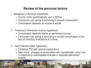
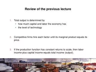
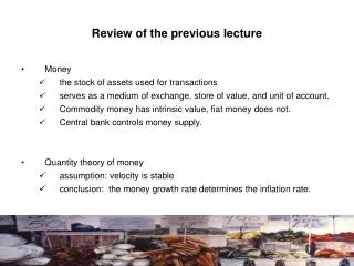
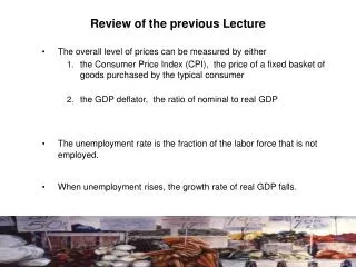
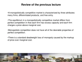
Review of the previous lecture The Solow growth model shows that, in the long run, a country’s standard of living depends positively on its saving rate. negatively on its population growth rate.
Lecture 7 Economic Growth – 1(B) Instructor: Prof. Dr.Qaisar Abbas
Lecture Contents Steady state Golden Rule
The equation of motion for k The Solow model’s central equation Determines behavior of capital over time… …which, in turn, determines behavior of all of the other endogenous variables because they all depend on k. E.g., income per person: y = f(k) consump. per person: c = (1–s) f(k) k = sf(k)– k
The steady state If investment is just enough to cover depreciation [sf(k)=k ], then capital per worker will remain constant: k = 0. This constant value, denoted k*, is called the steady state capital stock. k = sf(k)– k
The steady state Investment and depreciation k sf(k) k* Capital per worker, k
Moving toward the steady state Investment and depreciation k sf(k) k investment depreciation k1 k* Capital per worker, k k = sf(k) k
Moving toward the steady state Investment and depreciation k sf(k) k k* k1 Capital per worker, k k = sf(k) k k2
Moving toward the steady state Investment and depreciation k sf(k) k investment depreciation k* Capital per worker, k k = sf(k) k k2
Moving toward the steady state Investment and depreciation k sf(k) k k* Capital per worker, k k = sf(k) k k2 k3
Moving toward the steady state Investment and depreciation k sf(k) k* Capital per worker, k k = sf(k) k Summary:As long as k < k*, investment will exceed depreciation, and k will continue to grow toward k*. k3
A numerical example Production function (aggregate): To derive the per-worker production function, divide through by L: Then substitute y = Y/L and k = K/L to get
A numerical example, cont. Assume: s = 0.3 = 0.1 initial value of k = 4.0
Approaching the Steady State: A Numerical Example Year k y c i k k 1 4.000 2.000 1.400 0.600 0.400 0.200 2 4.200 2.049 1.435 0.615 0.420 0.195 3 4.395 2.096 1.467 0.629 0.440 0.189 4 4.584 2.141 1.499 0.642 0.458 0.184 … 10 5.602 2.367 1.657 0.710 0.560 0.150 … 25 7.351 2.706 1.894 0.812 0.732 0.080 … 100 8.962 2.994 2.096 0.898 0.896 0.002 … 9.000 3.000 2.100 0.900 0.900 0.000
Exercise: solve for the steady state Continue to assume s = 0.3, = 0.1, and y = k 1/2 Use the equation of motion k = s f(k) k to solve for the steady-state values of k, y, and c.
An increase in the saving rate Investment and depreciation k s2 f(k) s1 f(k) k An increase in the saving rate raises investment… …causing the capital stock to grow toward a new steady state:
Prediction Higher s higher k*. And since y = f(k) , higher k* higher y* . Thus, the Solow model predicts that countries with higher rates of saving and investment will have higher levels of capital and income per worker in the long run.
International Evidence on Investment Rates and Income per Person
The Golden Rule: introduction Different values of s lead to different steady states. How do we know which is the “best” steady state? Economic well-being depends on consumption, so the “best” steady state has the highest possible value of consumption per person: c* = (1–s) f(k*) An increase in s leads to higher k* and y*, which may raise c* reduces consumption’s share of income (1–s), which may lower c* So, how do we find the s and k* that maximize c* ?
The Golden Rule Capital Stock the Golden Rule level of capital,the steady state value of kthat maximizes consumption. To find it, first express c* in terms of k*: c* = y*i* = f (k*) i* = f (k*) k* In general: i= k + k In the steady state: i*=k* because k = 0.
The Golden Rule Capital Stock steady state output and depreciation k* f(k*) steady-state capital per worker, k* Then, graph f(k*) and k*, and look for the point where the gap between them is biggest.
The Golden Rule Capital Stock c*= f(k*) k*is biggest where the slope of the production func. equals the slope of the depreciation line: k* f(k*) MPK = steady-state capital per worker, k*
Use calculus to find golden rule We want to maximize: c*= f(k*) k* From calculus, at the maximum we know the derivative equals zero. Find derivative: dc*/dk*= MPK Set equal to zero: MPK = 0 or MPK =
The transition to the Golden Rule Steady State The economy does NOT have a tendency to move toward the Golden Rule steady state. Achieving the Golden Rule requires that policymakers adjust s. This adjustment leads to a new steady state with higher consumption. But what happens to consumption during the transition to the Golden Rule?
Starting with too much capital then increasing c* requires a fall in s. In the transition to the Golden Rule, consumption is higher at all points in time. time y c i t0
Starting with too little capital then increasing c* requires an increase in s. Future generations enjoy higher consumption, but the current one experiences an initial drop in consumption. y c i t0 time
Population Growth Assume that the population--and labor force-- grow at rate n. (n is exogenous) • EX: Suppose L = 1000 in year 1 and the population is growing at 2%/year (n = 0.02). Then L = n L = 0.02 1000 = 20, so L = 1020 in year 2.
Break-even investment ( + n)k = break-even investment, the amount of investment necessary to keep k constant. Break-even investment includes: k to replace capital as it wears out n k to equip new workers with capital(otherwise, k would fall as the existing capital stock would be spread more thinly over a larger population of workers)
The equation of motion for k With population growth, the equation of motion for k is k = s f(k) ( + n)k actual investment break-even investment
The Solow Model diagram Investment, break-even investment (+n)k sf(k) k* Capital per worker, k k=s f(k) ( +n)k
The impact of population growth (+n2)k sf(k) k2* Investment, break-even investment (+n1)k An increase in n causes an increase in break-even investment, leading to a lower steady-state level of k. k1* Capital per worker, k
Prediction Higher n lower k*. And since y = f(k) , lower k* lower y* . Thus, the Solow model predicts that countries with higher population growth rates will have lower levels of capital and income per worker in the long run.
International Evidence on Population Growth and Income per Person
The Golden Rule with Population Growth To find the Golden Rule capital stock, we again express c* in terms of k*: c* = y*i* = f (k* ) ( + n)k* c* is maximized when MPK = + n or equivalently, MPK = n In the Golden Rule Steady State, the marginal product of capital net of depreciation equals the population growth rate.
Summary An increase in the saving rate leads to higher output in the long run faster growth temporarily but not faster steady state growth.