Download
1 / 58
620 likes | 1.13k Views
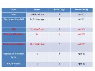
Lecture 20 Empirical Orthogonal Functions and Factor Analysis. Motivation in Fourier Analysis the choice of sine and cosine “patterns” was prescribed by the method. Could we use the data itself as a source of information about the shape of the patterns?.

E N D
Motivationin Fourier Analysis the choice of sine and cosine “patterns” was prescribed by the method.Could we use the data itself as a source of information about the shape of the patterns?
Examplemaps of some hypothetical function,say, sea surface temperatureforming a sequence in time
the data time time
pattern number pattern importance
Choose just the most important patterns pattern number pattern importance 3
comparison original reconstruction using only 3 patterns Note that this process has reduced the noise(since noise has no pattern common to all the images)
amplitudes of patterns time Note: no requirement that pattern is periodic in time
Useful tool for data that has three “components” ternary diagram C A B
works for 3 end-members, as long as A+B+C=100% C 0% A 25% A 50% A 75% A 100% A B … similarly for B and C
Suppose data fall near line on diagram C = data A B
Suppose data fall near line on diagram C = end-members or factors f1 f2 A B
Suppose data fall near line on diagram C = end-members or factors f1 f2 A B
50% Suppose data fall near line on diagram C = end-members or factors f1 mixing line f2 A B
C f1 f2 A B data idealize as being on mixing line
You could represent the data exactly with a third ‘noise’ factor C doesn’t much matter where you put f3, as long as it’s not on the line f1 f2 f3 A B
S: components (A, B, C, …) in each sample, s (A in s1) (B in s1) (C in s1) (A in s2) (B in s2) (C in s2) (A in s3) (B in s3) (C in s3) … (A in sN) (B in sN) (C in sN) S = N samplesM componentsS is NM Note: a sample is along a row in S
F: components (A, B, C, …) in each factor, f (A in f1) (B in f1) (C in f1) (A in f2) (B in f2) (C in f2) (A in f3) (B in f3) (C in f3) F = M componentsM factorsF is MM
C: coefficients of the factors (f1 in s1) (f2 in s1) (f3 in s1) (f1 in s2) (f2 in s2) (f3 in s2) (f1 in s3) (f2 in s3) (f3 in s3) … (f1 in sN) (f2 in sN) (f3 in sN) C = N samplesM factorsC is NM
SamplesNM S = C F (A in s1) (B in s1) (C in s1) (A in s2) (B in s2) (C in s2) (A in s3) (B in s3) (C in s3) … (A in sN) (B in sN) (C in sN) (f1 in s1) (f2 in s1) (f3 in s1) (f1 in s2) (f2 in s2) (f3 in s2) (f1 in s3) (f2 in s3) (f3 in s3) … (f1 in sN) (f2 in sN) (f3 in sN) (A in f1) (B in f1) (C in f1) (A in f2) (B in f2) (C in f2) (A in f3) (B in f3) (C in f3) = FactorsMM CoefficientsNM
SamplesNM data approximated with only most important factorsp most important factors = those with the biggest coefficients S C’ F’ (A in s1) (B in s1) (C in s1) (A in s2) (B in s2) (C in s2) (A in s3) (B in s3) (C in s3) … (A in sN) (B in sN) (C in sN) (f1 in s1) (f2 in s1) (f1 in s2) (f2 in s2) (f1 in s3) (f2 in s3) … (f1 in sN) (f2 in sN) (A in f1) (B in f1) (C in f1) (A in f2) (B in f2) (C in f2) = ignore f3 ignore f3 selectedcoefficientsNp selectedfactors pM
view samples as vectors in space B s1 s2 s3 Let the factors be unit vectors … f C A … then the coefficients are the projections (dot products) of the sample onto the factors
B s1 s2 s3 f C A Suggests a method of choosing factors so that they have large coefficients: Find the factor f that maximizesE = Si [ si f ]2with the constraint that ff =1Note: square the dot product since it can be negative
Find the factor f that maximizesE = Si [ si f ]2 with the constraint that L = ff – 1 = 0E = Si [ si f ]2 = Si [Sj Sij fj] [Sk Sik fk] = SjSk [Si Sij Sik] fj fk = SjSk Mjk fj fk with Mjk= Si Sij Sik or M=STSL = Si fi2 – 1Use Lagrange Multipliers, minimizing F=E-l2L, where l2 is the Lagrange Multiplier. We solved this problem 2 lectures ago. It’s solution is the algebraic eigenvalue problemMf = l2f. Recall that the eigenvalue is the corresponding value of E. symmetric Write as square for reasons that will become apparent later
So factors solve the algebraic eigenvalue problem:[STS] f = l2f.[STS]is a square matrix with the same number of rows and columns as there are components. So there are as many factors as there are components. The factors must span a space of the same dimension as the components.If you sort the eigenvectors by the size of their eigenvectors, then the ones with the largest eigenvalue have the largest components. So selecting the most important factors is easy.
An important tidbit from the theory of eigenvalues and eigenvectors that we’ll use later on …[STS] f = l2f.LetL2 be a diagonal matrix of eigenvalues, li2and letV be a matrix whose columns are the corresponding factors, f(i)Then[STS] = V L2 VT
Note also that the factors are orthogonalf(i)f(j)= 0 if ijThis is a mathematically pleasant propertyBut it may not always be the physically most-relevant choice close to mean of data contains negative A C C f2 f1 f1 f2 A not orthogonal B B orthogonal A
Upshoteigenvectors of [STS] f = l2f with the p eigenvaluesidentify a p-dimensional sub-spacein which most of the data lieyou can use those eigenvectors as factorsOrYou can chose any other p factors that span that subspace In the ternary diagram example, they must lie on the line connecting the two SVD factors
Singular Value Decomposition (SVD)Any NM matrix S and be written as the product of three matricesS = ULVTwhere U is NN and satisfies UTU = UUTV is MM and satisfies VTV = VVTandL is an NM diagonal matrix of singular values
Now note that itS = ULVT thenSTS = [ULVT]T [ULVT] = VLUTULVT =VL2VT Compare with the tidbit mentioned earlier STS=VL2VT The SVD V is the same V we were talking about earlierThe columns of V are the eigenvectors f, soF = VTSo we can use the SVD to calculatethe factors, F
But its even better than that! WriteS = ULVT asS = ULVT = [UL] [VT] = C FSo the coefficients are C = ULand, as shown previously, the factors areF = VTSo we can use the SVD to calculatethe coefficients, C, and the factors, F
MatLab Codefor computing C and F [U,LAMBDA,V] = svd(S); C = U*LAMBDA; F = V’;
MatLab Codeapproximating SSp using only the p most important factors p = (whatever); Up=U(:,1:p); LAMBDAp=LAMBDA(1:p,1:p); Cp = Up*LAMBDAp; Vp = V(:,1:p); Fp = (Vp)’; Sp = Cp * Fp;
Each pixel is a component of the imageand the patters are factorsour derivation assumed that the data (samples, s(i)) were vectorsHowever, in this example, the data are images (matrices)so what I had to do was to write out the pixels of each image as a vector
Steps1) load images2) reorganize images into S3) SVD of S to get UL and V4) Examine L to identify number of significant factors5) Build S’, using only significant factors6) reorganize S’ back into images
MatLab code for reorganizing a sequence of imagesD(p,q,r) (p=1 …Nx) (q=1 …Nx) (r=1 …Nt) into the sample matrix, S(r,s) (r=1 …Nt) (q=1 …Nx2) for r = [1:Nt] % time r for p = [1:Nx] % row p for q = [1:Nx] % col q s = Nx*(p-1)+q; % index s S(r,s) = D(p,q,r); end end end
MatLab code for reorganizing the sample matrixS(r,s) (r=1 …Nt) (s=1 …Nx2) back into a sequence of imagesD(p,q,r) (p=1 …Nx) (q=1 …Nx) (r=1 …Nt) for r = [1:Nt] % time p for s = [1:Nx*Nx] % index s p = floor( (s-1)/Nx+0.01 ) + 1; % row p q = s - Nx*(p-1); % col q D(p,q,r) = S(r,s); end end
Reality of Factorsare factors intrinsically meaningful, or just a convenient way of representing data? Example: Suppose the samples are rocks and the components are element concentrations then thinking of the factors as minerals might make intuitive sense Minerals: fixed element composition Rock: mixture of minerals
Many rocks – but just a few minerals rock 3 rock 1 rock 2 rock 6 rock 7 rock 5 mineral (factor) 1 rock 4 mineral (factor) 2 mineral (factor) 3
Possibly Desirable Properties of Factors Factors are unlike each other different minerals typically contain different elements Factor contains either large or near-zero components a mineral typically contains only a few elements Factors have only positive components minerals composed of positive amount of chemical elements Coefficient of factors are positive rocks composed of positive amount of minerals Coefficient typically either large or near-zero rocks composed of just a few major minerals
Transformations of Factors S = CF Suppose we mix factors together to get new factors set of factors (A in f1) (B in f1) (C in f1) (A in f2) (B in f2) (C in f2) (A in f3) (B in f3) (C in f3) (A in f’1) (B in f’1) (C in f’1) (A in f’2) (B in f’2) (C in f’2) (A in f’3) (B in f’3) (C in f’3) (f1 in f’1) (f2 in f’1) (f3 in f’1) (f1 in f’s2) (f2 in f’2) (f3 in f’2) (f1 in f’3) (f2 in f’3) (f3 in f’3) = New FactorsMM TransformationMM Old FactorsMM Fnew = TFold
Transformations of Factors Fnew = TFold A requirement is that T-1 exists, else Fnew will not span the same space as Fold S = CF = CIF = (CT-1) (T F)= Cnew Fnew So you could try to implement the desirable factors by designing an appropriate transformation matrix, T A somewhat restrictive choice of T is T=R, where R is a rotation matrix (rotation matrices satisfy R-1=RT)
A method for implementing this property Factors are unlike each other different minerals typically contain different elements Factor contains either large or near-zero components a mineral typically contains only a few elements Factors have only positive components minerals composed of positive amount of chemical elements Coefficient of factors are positive rocks composed of positive amount of minerals Coefficient typically either large or near-zero rocks composed of just a few major minerals
Factor contains either large or near-zero components More-or-less equivalent to Lots of variance in the amounts of components contained in the factor
Usual formula for variance for data, x sd2 = N-2 [ N Sixi2 - (Si xi)2 ] Application to factor, f sf2 = N-2 [ N Sifi4 - (Si fi2)2 ] Note that we are measuring the variance of the squares of the elements of , f. Thus a factor has large sf2 if the absolute-value of its elements has a lot of variation. The sign of the elements is irrelevant.