Download
1 / 85
860 likes | 951 Views
Relational Data Model. Lecture 3. Relational Model. Domain – a set of atomic values. Example: set of integers Data Type – Description of a form that domain values can be represented. Each domain has a null value

E N D
Relational Data Model Lecture 3
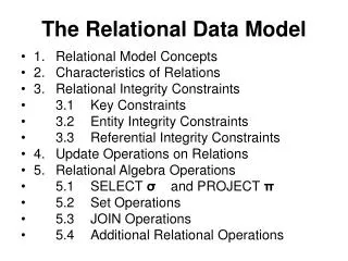
Relational Model • Domain – a set of atomic values. Example: set of integers • Data Type – Description of a form that domain values can be represented. Each domain has a null value • Cartesian Product – D1 x D2 a set of pairs <p1,p2> where p1 belongs to D1 and p2 belongs to D2. D1 x D2 x D3 x …x Dk –cartesian product of k domains. • Relation – a subset of the cartesian product of one or more domains. Elements of relation are called tuples. The number of domains in the relation is called relation arity • Relational Schema – a set of domain names along with theirs types. • Database – collection of relations • Database Schema – set of all relation schemas in the database
A Relation is a Table • Relation • Relational Scheme: Student(SSN, Name, Year) SSN Name Year 111-222-333 Jim senior 222-111-444 Jane junior 333-222-555 Joe freshman 213-343-565 Kyle junior
Relational Operators • Projection (R) • Natural join of R1 and R2 is a table that contains all attributes from R1 and from R1\R2 and tuples from r1 have the same values on attributes that are in both R1 and R2
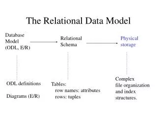
Reduction of an E-R Schema to Tables • Primary keys allow entity sets and relationship sets to be expressed uniformly as tables which represent the contents of the database. • A database which conforms to an E-R diagram can be represented by a collection of tables. • For each entity set and relationship set there is a unique table which is assigned the name of the corresponding entity set or relationship set. • Each table has a number of columns (generally corresponding to attributes), which have unique names.
Representing Entity Sets as Tables • A strong entity set reduces to a table with the same attributes.
Composite and Multivalued Attributes • Composite attributes are flattened out by creating a separate attribute for each component attribute • E.g. given entity set customer with composite attribute name with component attributes first-name and last-name the table corresponding to the entity set has two attributesname.first-name and name.last-name • A multivalued attribute M of an entity E is represented by a separate table EM • Table EM has attributes corresponding to the primary key of E and an attribute corresponding to multivalued attribute M • E.g. Multivalued attribute dependent-names of employee is represented by a tableemployee-dependent-names( employee-id, dname) • Each value of the multivalued attribute maps to a separate row of the table EM
Representing Relationship Sets as Tables • A many-to-many relationship set is represented as a table with columns for the primary keys of the two participating entity sets, and any descriptive attributes of the relationship set. • E.g.: table for relationship set borrower
Additional Rules for Translating Relationship into Relation If one entity set participates several times in the relationship with different roles, its key attributes must be listed as many times and with different names for each role. Studies(SSN, Name); Favorite(SSN, Name); Friends(SSN1, SSN2) Name SSN subject studies Student friends favorite
Redundancy of Tables • Many-to-one relationship sets that are total on the many-side can be represented by adding an extra attribute to the many side, containing the primary key of the one side • Example: We eliminate relation Favorite and we extend relation for Student as follows: Student(SSN, Name, Subject.name) • If, however, the relationship is many-to-many we cannot do that since it leads to redundancy For example relation Studies cannot be eliminated since otherwise we may end up with: 111-222-333 John OS 111-222-333 John DBMS
Representing Weak Entity Sets • A weak entity set becomes a table that includes a column for the primary key of the identifying strong entity set
Representing Weak Entity Sets(Additional Rules) • The relation for any relationship in which the weak W entity participates must use as a key for W all of its key attributes including those of strong entities that contribute to the W key • Weak entity set W participating in the relationship should not be converted into a relation.
Representing Specialization as Tables Form a table for the higher level entity Form a table for each lower level entity set, include primary key of higher level entity set and local attributes tabletable attributesperson name, street, city customer name, credit-ratingemployee name, salary • Drawback: getting information about, e.g., employee requires accessing two tables
Relations Corresponding to Aggregation • To represent aggregation, create a table containing • primary key of the aggregated relationship, • the primary key of the associated entity set • Any descriptive attributes
ssn Example name ISA person passenger age booked ISA date departure assigned pilot #fhrs gate instantof canfly flight plane dtime atime F# man model
Relational schema for the ER diagram • Passenger(ssn) Passenger(ssn, f#, date) • Departure(f#, date, gate) departure(f#,date,gate,man,model,ssn) • Booked(f#, ssn) • Flight(f#, dtime, atime) Flight(f#, dtime,atime) • Assigned(f#, man, model, ssn) • Person(ssn, name, age) Person(ssn,name,age) • Pilot(ssn, #hrs) Pilot(ssn,#hrs,man,model,f#,date) • Plane(man, model) Plane(man,model) • Canfly(man, model, ssn)
Functional Dependencies • Let R(A1, A2, ….Ak) be a relational schema; X and Y are subsets of {A1, A2, …Ak}. We say that X->Y, if any two tuples that agree on X, then they agree on Y. • Example: Student(SSN,Name,Addr,subjectTaken,favSubject,Prof) SSN->Name SSN->Addr subjectTaken->Prof Assign(Pilot,Flight,Date,Departs) Pilot,Date,Departs->Flight Flight,Date->Pilot
Functional Dependencies • No need for FD’s with more than one attribute on right side. But it maybe convenient: SSN->Name SSN->Addr combine into: SSN-> Name,Addr • More than one attribute on left is important and we may not be able to eliminate it. Flight,Date->Pilot
Functional Dependencies • A functional dependency X->Y is trivial if it is satisfied by any relation that includes attributes from X and Y • E.g. • customer-name, loan-number customer-name • customer-name customer-name • In general, is trivial if
Keys of Relations • X is a superkey of R if and only if X->R • X is a candidate key if X is a superkey and there is no subset of X that is also a superkey for R • One of the candidate keys is selected as a primary key • Example: SSN is a key for Student(SSN,NAME, ADDR) • How to determine keys of a relation: • One can assert a key K. Then the only FD on R is K->R • One can be given a set of FDs and keys can be found from these dependencies
Closure of a Set of Functional Dependencies • Given a set F set of functional dependencies, there are certain other functional dependencies that are logically implied by F. • E.g. If A B and B C, then we can infer that A C • The set of all functional dependencies logically implied by F is the closure of F. • We denote the closure of F by F+.
Closure of a Set of Functional Dependencies • An inference axiom is a rule that states if a relation satisfies certain FDs, it must also satisfy certain other FDs • Set of inference rules is sound if the rules lead only to true conclusions • Set of inference rules is complete, if it can be used to conclude every valid FD on R • We can find all ofF+by applying Armstrong’s Axioms: • if , then (reflexivity) • if , then (augmentation) • if , and , then (transitivity) • These rules are • sound and complete
Example • R = (A, B, C, G, H, I)F = { A BA CCG HCG IB H} • some members of F+ • A H • by transitivity from A B and B H • AG I • by augmenting A C with G, to get AG CG and then transitivity with CG I
To compute the closure of a set of functional dependencies F: F+ = Frepeatfor each functional dependency f in F+ apply reflexivity and augmentation rules on fadd the resulting functional dependencies to F+for each pair of functional dependencies f1and f2 in F+iff1 and f2 can be combined using transitivitythen add the resulting functional dependency to F+until F+ does not change any further Procedure for Computing F+
Closure of Functional Dependencies • We can further simplify manual computation of F+ by using the following additional rules. • If holds and holds, then holds (union) • If holds, then holds and holds (decomposition) • If holdsand holds, then holds (pseudotransitivity) The above rules can be inferred from Armstrong’s axioms.
Closure of Attribute Sets • Given a set of attributes a, define the closureof aunderF (denoted by a+) as the set of attributes that are functionally determined by a under F:ais in F+ a+ • Algorithm to compute a+, the closure of a under F result := a;while (changes to result) do for each in F do begin if result then result := result end
There are several uses of the attribute closure algorithm: Testing for superkey: To test if is a superkey, we compute +, and check if + contains all attributes of R. Testing functional dependencies To check if a functional dependency holds (or, in other words, is in F+), just check if +. That is, we compute + by using attribute closure, and then check if it contains . Is a simple and cheap test, and very useful Computing closure of F For each R, we find the closure +, and for each S +, we output a functional dependency S. Uses of Attribute Closure
Example of Attribute Set Closure • R = (A, B, C, G, H, I) • F = {A B, A C, CG H, CG I, B H} • (AG)+ 1. result = AG 2. result = ABCG (A C and A B) 3. result = ABCGH (CG H and CG AGBC) 4. result = ABCGHI (CG I and CG AGBCH) • Is AG a key? • Is AG a super key? • Does AG R? == Is (AG)+ R • Is any subset of AG a superkey? • Does AR? == Is (A)+ R • Does GR? == Is (G)+ R
Extraneous Attributes • Consider a set F of functional dependencies and the functional dependency in F. • Attribute A is extraneous in if A and (F – {}) {( – A) } logically implies F,or A and the set of functional dependencies (F – {}) {(– A)} logically implies F. • Example: Given F = {AC, ABC } • B is extraneous in AB C because {AC, AB C} logically implies AC (I.e. the result of dropping B from AB C). • Example: Given F = {AC, ABCD} • C is extraneous in ABCD since AB C can be inferred even after deleting C
Testing if an Attribute is Extraneous • Consider a set F of functional dependencies and the functional dependency in F. • To test if attribute A is extraneousin • compute ({} – A)+ using the dependencies in F • check that ({} – A)+ contains A; if it does, A is extraneous • To test if attribute A is extraneous in • compute + using only the dependencies in F’ = (F – {}) {(– A)}, • check that + contains A; if it does, A is extraneous
Canonical Cover • Sets of functional dependencies may have redundant dependencies that can be inferred from the others • Eg: A C is redundant in: {A B, B C, A C} • Parts of a functional dependency may be redundant • E.g. on RHS: {A B, B C, A CD} can be simplified to {A B, B C, A D} • E.g. on LHS: {A B, B C, AC D} can be simplified to {A B, B C, A D} • A canonical cover of F is a “minimal” set of functional dependencies equivalent to F, having no redundant dependencies or redundant parts of dependencies
Canonical Cover(Formal Definition) • A canonical coverfor F is a set of dependencies Fc such that • F logically implies all dependencies in Fc, and • Fclogically implies all dependencies in F, and • No functional dependency in Fc contains an extraneous attribute, and • Each left side of functional dependency in Fcis unique.
Canonical CoverComputation • To compute a canonical cover for F:repeatUse the union rule to replace any dependencies in F11 and 11 with 112 Find a functional dependency with an extraneous attribute either in or in If an extraneous attribute is found, delete it from until F does not change
Example of Computing a Canonical Cover • R = (A, B, C)F = {A BC B C A BABC} • Combine A BC and A B into A BC • A is extraneous in ABC • Set is now {A BC, B C} • C is extraneous in ABC • Check if A C is logically implied by A B and the other dependencies • Yes: using transitivity on A B and B C. • The canonical cover is: A B B C
Foreign Keys • Let R1 and R2 be two relational schemas. Let K1 and K2 be primary keys of R1 and R2, respectively. If R1 contains all attributes from K2, then we say that K2 is a foreign key of R1. • Integrity Constraints • Domain Constraints • Key Constraints • Interdomain Constraints • Database Schema S is a set of relational schemas and constraints defined on them
Constraints • Insert Constraints: • No tuple should be inserted into a relation r1 with foreign keys of r2 that are not listed as primary key in r2 (referential integrity) • No tuples should be inserted with duplicate primary key(primary key constraint) • No primary key value can contain nulls (primary key constraint) • Delete Constraint: Tuple should not be deleted from r2 with foreign key values for r2, if a deletion of this tuple will result in referential integrity constraint violation • Update should respect referential and primary key constraints
Relational Database Design Problem • Problem: Given a set of attributes and a set of FDs, generate a set of relational schemas describing the enterprise. • Approach 1: Make one big relational schema that contains all attributes (universal relation approach) • Problems: • Repetition of information (name, addr, dep_name): address is repeated for each dependent. • Inability to represent certain information, unless nulls are used (name, position,sal, comission) • Loss of information: referential integrity violations
Relational Database Design Problem • If one big relational schema is not good, then we need to decompose it into smaller relational schemas so that no loss of information will occur • Issue: how to decompose without loosing the information? (person_name, loan#, balance, branch_name) Decompose into: (person_name,loan#) (loan#,balance,branch_name) Information gets lost! • Thus, we need to find a lossless decomposition
Decomposition • All attributes of an original schema (R) must appear in the decomposition (R1, R2): R = R1 R2 • Lossless-join decomposition.For all possible relations r on schema R r = R1 (r) R2 (r) • A decomposition of R into R1 and R2 is lossless join if and only if at least one of the following dependencies is in F+: • R1 R2R1 • R1 R2R2
Example of Lossy-Join Decomposition • Lossy-join decompositions result in information loss. • Example: Decomposition of R = (A, B) R1 = (A) R2 = (B) A B A B 1 2 1 1 2 B(r) A(r) r A B A (r) B (r) 1 2 1 2
Goals of Normalization • Decide whether a particular relation R is in “good” form. • In the case that a relation R is not in “good” form, decompose it into a set of relations {R1, R2, ..., Rn} such that • each relation satisfies a referential integrity constraints • the decomposition is a lossless-join decomposition • the decomposition preserves the set of functional dependencies • Our theory initially is based on: • functional dependencies
Normalization Using Functional Dependencies • When we decompose a relation schema R with a set of functional dependencies F into R1, R2,.., Rn we want • Lossless-join decomposition: Otherwise decomposition would result in information loss. • Dependency preservation: Let Fibe the set of dependencies F+ that include only attributes in Ri. (F1 F2 … Fn)+ = F+ .
Example • R = (A, B, C)F = {A B, B C) • Can be decomposed in two different ways • R1 = (A, B), R2 = (B, C) • Lossless-join decomposition: R1 R2 = {B} and B BC • Dependency preserving • R1 = (A, B), R2 = (A, C) • Lossless-join decomposition: R1 R2 = {A} and A AB • Not dependency preserving (cannot check B C without computing R1 R2)
To check if a dependency is preserved in a decomposition of R into R1, R2, …, Rn we apply the following simplified test (with attribute closure done w.r.t. F) result = while (changes to result) dofor eachRiin the decompositiont = (result Ri)+ Riresult = result t If result contains all attributes in , then the functional dependency is preserved. We apply the test on all dependencies in F to check if a decomposition is dependency preserving This procedure takes polynomial time, instead of the exponential time required to compute F+and(F1 F2 … Fn)+ Testing for Dependency Preservation
Boyce-Codd Normal Form A relation schema R is in BCNF with respect to a set F of functional dependencies if for all functional dependencies in F+ of the form , where R and R,at least one of the following holds: • is trivial (i.e., ) • is a superkey for R
Example • R = (A, B, C)F = {AB B C}Key = {A} • R is not in BCNF • Decomposition R1 = (A, B), R2 = (B, C) • R1and R2 in BCNF • Lossless-join decomposition • Dependency preserving
Testing for BCNF • To check if a non-trivial dependency causes a violation of BCNF 1. compute + (the attribute closure of ), and 2. verify that it includes all attributes of R • Using only F is incorrect when testing a relation in a decomposition of R • E.g. Consider R (A, B, C, D), with F = { A B, B C} • Decompose R into R1(A,B) and R2(A,C,D) • Neither of the dependencies in F contain only attributes from (A,C,D) so we might be mislead into thinking R2 satisfies BCNF. • In fact, dependency AC in F+ shows R2 is not in BCNF.
BCNF Decomposition Algorithm result := {R};done := false;compute F+;while (not done) do if (there is a schema Riin result that is not in BCNF)then beginlet be a nontrivial functional dependency that holds on Ri such that Riis not in F+, and = ;result := (result – Ri ) (Ri – ) (, );end else done := true; Each Riis in BCNF, and decomposition is lossless-join.
Example of BCNF Decomposition • R = (branch-name, branch-city, assets, customer-name, loan-number, amount) F = {branch-name assets branch-city loan-number amount branch-name} Key = {loan-number, customer-name} • Decomposition • R1 = (branch-name, branch-city, assets) • R2 = (branch-name, customer-name, loan-number, amount) • R3 = (branch-name, loan-number, amount) • R4 = (customer-name, loan-number) • Final decomposition R1, R3, R4
BCNF and Dependency Preservation It is not always possible to get a BCNF decomposition that is dependency preserving • R = (A, B, C)F = {AB C C B}Two candidate keys = ABand AC • R is not in BCNF • Any decomposition of R will fail to preserve AB C