Minimum Spanning Trees

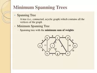
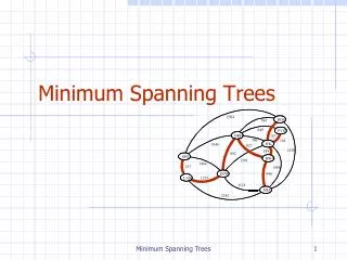
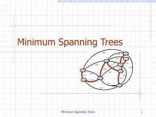
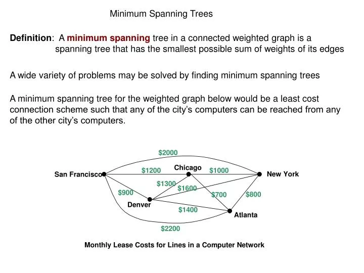
Minimum Spanning Trees Definition: A minimum spanning tree in a connected weighted graph is a spanning tree that has the smallest possible sum of weights of its edges A wide variety of problems may be solved by finding minimum spanning trees A minimum spanning tree for the weighted graph below would be a least cost connection scheme such that any of the city’s computers can be reached from any of the other city’s computers.

Example

Kruskal’s Minimum Spanning Tree Algorithm The first minimum spanning tree algorithm we will discuss is Kruskal’s Algorithm The basis of Kruskal’s Algorithm is the following characterization of a tree: Graph T with n vertices is a tree if and only if T contains no cycles and has exactly n-1 edges An acyclic graph on n vertices with fewer than n-1 edges must be disconnected. Each connected component of such a graph will be a tree. Such a graph is called a forest. Actually, the formal definition of a forest allows for the possibility of a single tree.

Kruskal’s Minimum Spanning Tree Algorithm Each connected component of a forest is a tree. If F is a forest, the component partition of its vertex set consists of the vertex sets of its component trees.

Kruskal’s Minimum Spanning Tree Algorithm Each connected component of a forest is a tree. If F is a forest, the component partition of its vertex set consists of the vertex sets of its component trees. The component partition of the above forest is { {a,f}, }

Kruskal’s Minimum Spanning Tree Algorithm Each connected component of a forest is a tree. If F is a forest, the component partition of its vertex set consists of the vertex sets of its component trees. The component partition of the above forest is { {a,f}, {d,g,i,j}, }

Kruskal’s Minimum Spanning Tree Algorithm Each connected component of a forest is a tree. If F is a forest, the component partition of its vertex set consists of the vertex sets of its component trees. The component partition of the above forest is { {a,f}, {d,g,i,j}, {b}, }

Kruskal’s Minimum Spanning Tree Algorithm Each connected component of a forest is a tree. If F is a forest, the component partition of its vertex set consists of the vertex sets of its component trees. The component partition of the above forest is { {a,f}, {d,g,i,j}, {b},{c,e,h} }

Kruskal’s Minimum Spanning Tree Algorithm Each connected component of a forest is a tree. If F is a forest, the component partition of its vertex set consists of the vertex sets of its component trees. The component partition of the above forest is { {a,f}, {d,g,i,j}, {b}, {c,e,h} }

Kruskal’s Minimum Spanning Tree Algorithm How will the partition change if we add a new edge to the forest below connecting vertices a and d? Forest F Component Partition: { {a,f}, {d,g,i,j}, {b}, {c,e,h} } Forest F = F  { (a,d) } Component Partition: { {a,f,d,g,i,j}, {b}, {c,e,h} } The answer: the trees that been joined form a single tree, so the two component partition elements are combined to form one set

Kruskal’s Minimum Spanning Tree Algorithm The preceding suggests a way to build a spanning tree of a graph G Start with the spanning forest of G having no edges Forest F0 10 components Component Partition: { {a}, {b}, {c}, {d}, {e}, {f}, {g}, {h}, {i}, {j} }

Kruskal’s Minimum Spanning Tree Algorithm Then add one edge at a time so that a cycle is never created: Forest F1 9 components Component Partition: { {a}, {c}, {b, d}, {e}, {f}, {g}, {h}, {i}, {j} }

Kruskal’s Minimum Spanning Tree Algorithm Then add one edge at a time so that a cycle is never created: Forest F2 8 components Component Partition: { {a}, {c}, {b, d}, {e,j}, {f}, {g}, {h}, {i} }

Kruskal’s Minimum Spanning Tree Algorithm Then add one edge at a time so that a cycle is never created: Forest F3 7 components Component Partition: { {c}, {a,b,d} , {e,j}, {f}, {g}, {h}, {i} }

Kruskal’s Minimum Spanning Tree Algorithm Then add one edge at a time so that a cycle is never created: Forest F6 4 components Component Partition: { {c,h} , {a,b,d} , {e,j}, {f,g,i} }

Kruskal’s Minimum Spanning Tree Algorithm Then add one edge at a time so that a cycle is never created: Forest F9 1 components Component Partition: { {c,h,a,b,d,e,j,f,g,i} }

Kruskal’s Minimum Spanning Tree Algorithm How can we know if adding an edge will create a cycle? Answer: cycle is created  both endpoints in the same component tree   both endpoints in the same partition set Thus we know that at this point we cannot add edge {a,b} because they lie in the same set {a,b,d} in the component partition. Forest F6 4 components Component Partition: { {c,h} , {a,b,d} , {e,j}, {f,g,i} }

Simple Spanning Tree Algorithms Forest-to-Spanning-Tree Algorithm(G) n = number of vertices of G x = number of edges of G E = list of edges of the graph j = 1 // list traversal index i = 0 // number of edges added so far P = single-point partition of V(G) while i < n-1 and j <= x: // don’t have a tree and have more edges to examine {u,v} = E[j] // get next edge // Skip over edges within a component tree while j <= x and u and v lie in the same set in P: j = j+1 {u,v} = E[j] if j <= x add {u,v} to the edge set of T delete from P set U containing u and set V containing v add U union V to P if i < n-1 print “this graph is not connected” else return T

Kruskal’s Algorithm Kruskal’s greedy algorithm adds the caveat that the edges that are added in the general Forest-To-Tree Algorithm should have been sorted into non-decreasing weight order Thus, one could give the following abstract description of Kruskal’s algorithm: Kruskal: T  a minimum-weight edge; for ( i = 1 to n-2) { e  a minimum weight edge not in T that does not create a simple cycle when added to T T  T + e }

Implementing Kruskal’s Algorithm • Kruskal’s algorithm is fairly simple conceptually • It is not hard to follow the algorithm for a specific weighted graph • But what makes the algorithm work is the underlying data structures used to carry out the critical step where a new edge is chosen for the forest • We will illustrate the geometric tracing of the algorithm first • We will then show how the data structures are used. This is critical to an understanding of the complexity of the algorithms

Example: Kruskal’s Algorithm We will illustrate Kruskal’s Algorithm by applying it to our computer network.

Example: Kruskal’s Algorithm T  a minimum-weight edge; {Chicago,Atlanta}

Example: Kruskal’s Algorithm T  T + a minimum-weight edge not in T whose addition creates no cycle {Chicago,Atlanta}, {Atlanta, New York}

Example: Kruskal’s Algorithm T  T + a minimum-weight edge not in T whose addition creates no cycle {Chicago,Atlanta}, {Atlanta, New York}, {Denver, San Francisco}

Example: Kruskal’s Algorithm T  T + a minimum-weight edge not in T whose addition creates no cycle {Chicago,Atlanta}, {Atlanta, New York}, {Denver, San Francisco}, {Chicago, San Francisco},

Kruskal’s Algorithm The preceding statement of Kruskal’s algorithm ignores implementation details, which we address at this time Three issues must be dealt with: > how do we represent the weighted graph > how do we choose a least cost edge > how do we decide if an edge forms a cycle with edges already included in our subgraph? Representation: use a list of edges and their weights Choosing least cost edge: sort the edge list by increasing weight and step through the list.

Kruskal’s Algorithm How do we decide if an edge forms a cycle with edges already included in our subgraph? Maintain a partition of the vertex set in which each set in the partition is the vertex set of a component of the current subgraph An edge forms a cycle when both of its endpoints lie in the same component If the edge does not form a cycle, then adding that edge to the forest combines the two underlying trees into a single tree The result of combining the two trees into one is that we replace the two partition sets by their union. So we need an efficient data structure for representing partitions of a set that efficiently supports > finding which set contains a given element ; and > taking the union of two sets in the partition This a problem studied in other settings and the algorithms are called Union-Find algorithms

Disjoint Sets • We now consider a data structure that maintains a collection of pair-wise disjoint sets • The required operations are • creating a set containing a single, given element; • taking the union of two of the sets; and • finding the set which contains a given element • We name a set by “marking” one of its elements as its representative • Then the operations are named as follows: • makeset(i) creates the set {i} with i as the marked element • union(i,j) merges the set containing i with the set containing j to form a new set, so that there is one fewer set than before. The marked element of one of the two sets becomes the marked element for the union • findset(i) returns the marked element of the set containing i

Example • makeset(1) makeset(2) makeset(3) makeset(4) makeset(5) • We now have the sets {1}, {2}, {3}, {4}, {5} • union(1,4) union(3,5) • The sets are now {1,4}, {2}, {3,5} • If we assume that 4 is the marked element of {1,4}, then findset(1) and findset(4) both return 4 • We can use findset to test if two elements lie in the same set:findset(1) == findset(4) returns true, findset(2) == findset(5)false • After the operation union(4,2) , we have {1,2,4}, {3,5} • If we then execute union(1,5) we are left with {1,2,3,4,5} • The value of findset is now the same for all elements

5 5 5 2 8 4 2 4 8 8 2 4 Tree Representation • We will represent a set by a rooted tree with the marked element at the root • Note: this has not the same as spanning trees of graphs • The trees are not arranged in any particular way; they are not, for example, binary trees • Here are three different trees that could be used to represent the set {2,4,5,8}, with 5 as the marked element:

Parent Array Representation of a Forest • We can represent a collection of disjoint trees (a forest) by means of an array parent such that: • parent[i] = i if i is a root, and is the value at the parent of i otherwise • Let {1,2,4,6}, {3,5} be our collection of disjoint sets with 2 and 5 marked • Then the tree representation might be: • The corresponding parent array would be 2 5 6 1 3 4 i parent[i]

First Version of Operations • makeset1(i) { parent[i] = i;} • findset1(i) { while( i  parent[i]) i = parent[i]; return i;} • union1(i,j) { a = findset1(i); b = findset1(j); parent[a] = b;}

Example Union1(10,20) {a = findset1(10); b = findset1(20); parent[5] = 18; a = 5 b = 18

Running Time: First Version • Typically, the disjoint set operations are run many times • We assume that n makeset operations are executed, followed by m findset and union operations • Each makeset1 call is (1), to the total for makeset1 is (n) • The worst-case running time of findset1 is the height of the tree in which we are searching • The most this can be is n-1, hence the the running time is O(n) • The running time for union1 is dominated by the two calls to findset1, and hence is also O(n) • This gives us a total running time for all the calls of O(n+mn) • We can refine this a bit: if m < n, then the max height is m, which could happen if all of the m calls were to union1 • In this case we get O(n+m2), and in any case we have O(n+mmin(m,n))

Improving the Performance • From the preceding run-time analysis, we could improve the running time if we could limit the depth of the trees • The worst thing we can do is to make the root of a shorter tree the parent of the root of a longer tree when doing a union. • If we have two trees of differing heights and we make the root of the deeper tree the root of the union, the height of the union equals the height of the deeper tree • If both trees have the same height, we increase the height by one • To implement this idea, we maintain another array to store the tree heights

Version 2 • makeset2(i) { parent[i] = i; height[i] = 0;} • findset2(i) is the same as findset1(i) • union2(i,j) { a = findset2(i); b = findset2(j); if (height(a) < height(b)) parent[a] = b; else if (height(b) < height(a)) parent[b] = a; else { parent[a] = b; height[b] = height[b] + 1; }}

Example height(5) = 4 height(18) = 3 Union2(10,20) {a = findset2(10); b = findset2(20); parent[18] = 5; a = 5 b = 18

Version 2 Running Time TheoremUsing version 2 of the disjoint-set algorithms, the height of a k-node tree is at most lg k Proof (by induction on k) Basis: If k = 1, then the tree has height 0 = lg 1 Inductive Step: Suppose k > 1 and the result holds for all p < k A k-node tree T is the union of two trees T1 and T2 since k > 1. If ki is the number of nodes in Ti and hi is the height of Ti, then hi  lg ki ( i = 1, 2 ) by the inductive hypothesis Moreover, k = k1 + k2 and, if h is the height of T, max{h1,h2} if h1 h2h = h1 + 1 if h1 = h2

Version 2 Running Time k = k1+ k2 and, if h is the height of T, max{h1,h2} if h1  h2h = h1 + 1 if h1 = h2 max{h1,h2}  max{lg k1, lg k2 } lg k Thus we may assume h1 = h2Without loss of generality we may also assume k1  k2 This implies that k2  k/2, since k1+k2 = k Thus h = 1 + h2  1 + lg k2 < 1 + lg k/2 = 1 + (lg k -1) = lg k inductive hypothesis each ki k = k1+k2

Run-Time Analysis of Version 2 • We may now mimic the arguments used in analyzing version 1 to obtain the running time for the version 2 algorithms:O(n + mmin{lg n, lg m})

A Final Improvement • There is one more trick we can use to improve performance • Every time we execute findset, we traverse a path from a node to the root of one of our trees • We can now retraverse the path, changing the parent of each of the nodes on the path to the root. • We will retain the union methodology from version 2, but we should not call the extra array the height array • Instead, that array will maintain an upper bound on the height, since path compression might make the height less than before • Thus, the additional information being kept will be called the rank of the vertex

Disjoint Sets, Version 3 makeset3(i) { parent[i] = i; rank[i] = 0;} findset3(i) { root = i; while (root != parent[root]) root = parent[root]; j = parent[i]; while j != root { parent[i] = root; i = j; j = parent[i]; } return root;}

Example rank(5) = 5 rank(18) = 3 Union3(10,20) {root = findset1(10);

root Example rank(5) = 5 rank(18) = 3 Union3(5,20) {root = findset3(10); root = 5

Example rank(5) = 5 rank(18) = 3 Union3(5,20) {root = findset3(10); root = 5

Example rank(5) = 5 rank(18) = 3 Union3(5,20) {root = findset3(10); b = findset3(20); root = 5 b = 18

Example rank(5) = 5 Union3(5,20) {root = findset1(10); b = findset3(20); parent[18] = 5; root = 5 b = 18

Minimum Spanning Trees