Download
1 / 25
250 likes | 314 Views
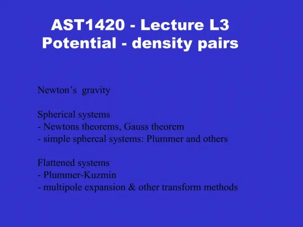
ASTC22 - Lecture L4 Potential - density pairs (continued). Flattened systems - Plummer-Kuzmin - multipole expansion & other transform methods There is nothing more practical than theory: - Gauss theorem in action - using v = sqrt(GM/r).

E N D
ASTC22 - Lecture L4 Potential - density pairs (continued) Flattened systems - Plummer-Kuzmin - multipole expansion & other transform methods There is nothing more practical than theory: - Gauss theorem in action - using v = sqrt(GM/r)
Very frequently used:spherically symmetric Plummer pot. (Plummer sphere) Notice and remember how the div grad (nabla squared or Laplace operator in eq. 2-48) is expressed as two consecutive differentiations over radius! It’s not just the second derivative. Constant b is known as the core radius. Do you see that inside r=b rho becomes constant?
Axisymmetric potential: Kuzmin disk model This is the so-called Kuzmin disk. It’s somewhat less useful than e.g., Plummer sphere, but hey… it’s a relatively simple potential - density (or rather surface density) pair.
Often used because of an appealingly flat rotation curve v(R)--> const at R--> inf
Useful approx. to galaxies if flattening is small
Not very useful approx. to galaxies if flattening not <<1, i.e. q not close to 1
This is how the Poisson eq looks like in cylindrical coord. (R,phi, theta) when nothing depends on phi (axisymmetric density). Simplified Poisson eq.for very flat systems. This equation was used in our Galaxy to estimate the amount of material (the r.h.s.) in the solar neighborhood.
Poisson equation: Multipole expansion method. This is an example of a transform method: instead of solving Poisson equation in the normal space (x,y,z), we first decompose density into basis functions (here called spherical harmonics Yml) which have corresponding potentials of the same spatial form as Yml, but different coefficients. Then we perform a synthesis (addition) of the full potential from the individual harmonics multiplied by the coefficients [square brackets] We can do this since Poisson eq. is linear.
In case of spherical harmonic analysis, we use the spherical coordinates. This is dictated by the simplicity of solutions in case of spherically symmetric stellar systems, where the harmonic analysis step is particularly simple. However, it is even simpler to see the power of the transform method in the case of distributions symmetric in Cartesian coordinates. An example will clarify this.
Example: Find the potential of a 3-D plane density wave (sinusoidal perturbation of density in x, with no dependence on y,z) of the form We use complex variables (i is the imaginary unit) but remember that the physical quantities are all real, therefore we keep in mind that we need to drop the imaginary part of the final answer of any calculation. Alternatively, and more mathematically correctly, we should assume that when we write any physical observable quantity as a complex number, a complex conjugate number is added but not displayed, so that the total of the two is the physical, real number (complex conjugate is has the same real part and an opposite sign of the imaginary part.) You can do it yourself, replacing all exp(i…) with cos(…). Before we substitute the above density into the Poisson equation, we assume that the potential can also be written in a similar form
Now, substitution into the Poisson equation gives where k = kx, or the wavenumber of our density wave. We thus obtained a very simple, algebraic dependence of the front coefficients (constant in terms of x,y,z, but in general depending on the k-vector) of the density and the potential. In other words, whereas the Poisson equation in the normal space involves integration (and that can be nasty sometimes), we solved the Poisson equation in k-space very easily. Multiplying the above equation by exp(…) we get the final answer As was to be expected, maxima (wave crests) of the 3-D sinusoidal density wave correspond to the minima (wave troughs, wells) of its gravitational potential. x
The second part of the lecture is a repetition of the useful mathematical facts and the presentation of several problems
This problem is related to Problem 2.17 on p. 84 of the Sparke/Gallagher textbook.