Download
1 / 45
450 likes | 784 Views
Sound and Speech Recognition. What is Sound ?. Acoustics is the study of sound. Physical - sound as a disturbance in the air Psychophysical - sound as perceived by the ear Sound as stimulus (physical event) & sound as a sensation. Pressures changes (in band from 20 Hz to 20 kHz)

E N D
What is Sound ? Acoustics is the study of sound. • Physical - sound as a disturbance in the air • Psychophysical - sound as perceived by the ear • Sound as stimulus (physical event) & sound as a sensation. • Pressures changes (in band from 20 Hz to 20 kHz) Physical terms • Amplitude • Frequency • Spectrum
Sound Waves • In a free field, an ideal source of acoustical energy sends out sound of uniform intensity in all directions. => Sound is propagating as a spherical wave. • Intensity of sound is inversely proportional to the square of the distance (Inverse distance law). • 6 dB decrease of sound pressure level per doubling the distance.
How we hear • Ear connected to the brain • left brain: speech • right brain: music • Ear's sensitivity to frequency is logarithmic • Varying frequency response • Dynamic range is about 120 dB (at 3-4 kHz) • Frequency discrimination 2 Hz (at 1 kHz) • Intensity change of 1 dB can be detected.
Digital Sampling • Sampling is dictated by the Nyquist sampling theorem which states how quickly samples must be taken to ensure an accurate representation of the analog signal. • The Nyquist sampling theorem states that the sampling frequency must be two times greater than the highest frequency in the original analog signal. or
Dithering a Sampled Signal • Analog signal added to the signal to remove the artifacts of quantization error. • Dither causes the audio signal to always move between quantization levels. • Otherwise, a low level signal would be encoded as a square wave => granulation noise. • Dithered, the A/D converter output is signal + noise => perceptually preferred, since noise is better tolerated than distortion. • Amplitude of dither signal: high dither amplitudes more easily remove quantization artifacts too much dither decreases the signal-to-noise ratio
Common Sound Sampling Parameters • Common Sampling Rates • 8KHz (Phone) or 8.012820513kHz (Phone, NeXT) • 11.025kHz (1/4 CD std) • 16kHz (G.722 std) • 22.05kHz (1/2 CD std) • 44.1kHz (CD, DAT) • 48kHz (DAT) • Bits per Sample • 8 or 16 • Number of Channels • mono/stereo/quad/ etc.
Space/Storage Requirements 1 Minute of Sound
Many (!) Sound File Formats • Mulaw (Sun, NeXT) .au • RIFF (Resource Interchange File Format) • MS WAV and .AVI • MPEG Audio Layer (MPEG) .mpa .mp3 • AIFC (Apple, SGI) .aiff .aif • HCOM (Mac) .hcom • SND (Sun, NeXT) .snd • VOC (Soundblaster card proprietary standard) .voc • AND MANY OTHERS!
What’s in a Sound File Format • Header Information • Magic Cookie • Sampling Rate • Bits/Sample • Channels • Byte Order • Endian • Compression type • Data
Example File Format (NIST SPHERE) NIST_1A 1024 sample_rate -i 16000 channel_count -i 1 sample_n_bytes -i 2 sample_byte_format -s2 10 sample_sig_bits -i 16 sample_count -i 594400 sample_coding -s3 pcm sample_checksum -i 20129 end_head
WAV file format (Microsoft) RIFF A collection of data chunks. Each chunk has a 32-bit Id followed by a 32-bit chunk length followed by the chunk data. 0x00 chunk id 'RIFF' 0x04 chunk size (32-bits) 0x08 wave chunk id 'WAVE' 0x0C format chunk id 'fmt ' 0x10 format chunk size (32-bits) 0x14 format tag (currently pcm) 0x16 number of channels 1=mono, 2=stereo 0x18 sample rate in hz 0x1C average bytes per second 0x20 number of bytes per sample 1 = 8-bit mono 2 = 8-bit stereo or 16-bit mono 4 = 16-bit stereo 0x22 number of bits in a sample 0x24 data chunk id 'data' 0x28 length of data chunk (32-bits) 0x2C Sample data
Digital Audio Today • Analog elements in the audio chain are replaced with digital elements. • 16-bit wordlength, 32/44.1/48 kHz sampling rates. • Mostly linear signal processing. • Wide range of digital formats and storage media. • Rapid development of technology => better SNR, phase and linearity. • Rapid increase of signal processing power => possibility to implement new, complex features. • Soon: Digital radio (satellite), HDTV
Digital (CD) vs Analog (LP or cassette tape) • Information is stored digitally. • The length of its data pits represents a series of 1s and 0s. • Both audio channels are stored along the same pit track. • Data is read using laser beam. • Information density about 100 times greater than in LP. • CD player can correct disc errors.
Benefits of Digital Representation (CD) • Robust • No degradation from repeated playings because data is read by the laser beam. • Error correction • Transport’s performance does not affect the quality of audio reproduction. • Digital circuitry more immune to aging and temperature problems • Data conversion is independent of variations in disc rotational speed, hence wow and flutter are negligible. • SNR over 90 dB. • Subcode for display, control and user information
CD Format • Sampling • 44.1 kHz => 10 % margin with respect to the Nyquist frequency (audible frequencies below 20 kHz) • 16-bit linear => theoretical SNR about 98 dB (for sinusoidal signal with maximum amplitude) • audio bit rate 1.41 Mbit/s (44.1 kHz * 16 bits * 2 channels) • Cross Interleaved Reed-Solomon Code (CIRC) for error correction • Subcode • Original Specifications • Playing time max. 74.7 min • Disc diameter 120 mm • Disc thickness 1.2 mm • One sided medium, rotates clockwise • Signal is recorded from inside to outside • Pit is about 0.5 µm wide • Pit edge is 1 and all other areas whether inside or outside a pit, are 0s
Acoustic Origins • A wave for the words “speech lab” looks like: s p ee ch l a b “l” to “a” transition: Graphs from Simon Arnfield’s web tutorial on speech, Sheffield: http://lethe.leeds.ac.uk/research/cogn/speech/tutorial/
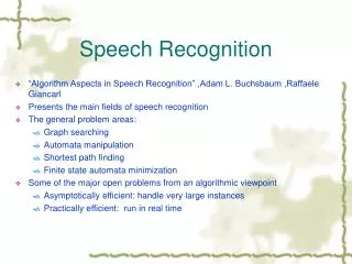
Acoustic Modeling Describes the sounds that make up speech Speech Recognition Lexicon Describes which sequences of speech sounds make up valid words Language Model Describes the likelihood of various sequences of words being spoken Speech Recognition Knowledge Sources
Speech Recognition THE FUNDAMENTAL EQUATION O is an acoustical ‘Observation’ w is a ‘word’ we are trying to recognize Maximize w = argmax (P(W) | O) P(W|O) is unknown so by Bayes’ rule: P(O|W) P(W) P(W|O) = ------------------------ P(O)
x x 1 T P ( x x w w ) P ( w w ) ... ... ... | ・ 1 T 1 k 1 k Mechanism of state-of-the-art speech recognizers Speech in Acoustic analysis ... P ( x x w w ) ... | ... 1 T 1 k Recognition: Maximize Pronunciation lexicon P ( w w ) ... 1 k Language model Recognized Sentence
Acoustic Sampling • 10 ms frame (ms = millisecond = 1/1000 second) • ~25 ms window around frame to smooth signal processing 25 ms . . . 10ms Result: Acoustic Feature Vectors a1 a2 a3
Spectral Analysis • Frequency gives pitch; amplitude gives volume • sampling at ~8 kHz phone, ~16 kHz mic (kHz=1000 cycles/sec) • Fourier transform of wave yields a spectrogram • darkness indicates energy at each frequency • hundreds to thousands of frequency samples s p ee ch l a b amplitude frequency
Features for Speech Recognition Coding scheme (typical) • 10 millisecond step size; 25 millisecond window • ~39 coefficients each step: • mel-scale cepstra derived from frequency representation • and coefficients • power
The Markov Assumption • Only immediately preceding history matters
S1 S2 S3 Hidden Markov Models • In speech recognition the number of states is very large; we can simplify the problem by factoring the problem into two components
Lexicon - links words to phones in acoustic model Aaron EH R AX N Aaron(2) AE R AX N abandon AX B AE N D AX N abandoned AX B AE N D AX N DD abandoning AX B AE N D AX N IX NG abandonment AX B AE N D AX N M AX N TD abated AX B EY DX IX DD abatement AX B EY TD M AX N TD abbey AE B IY Abbott AE B AX TD Abboud AA B UW DD abby AE B IY abducted AE BD D AH KD T IX DD Abdul AE BD D UW L
Language Models A language model is a probability distribution over word sequences • n = 3,4,5 [lose the rest of the context] • Hard to estimate large contexts: consider 64,000^3 words • Need large collections of text • Smoothing P(wi| wi-2, wi-1) is necessary
Creating models for recognition Speech data Acoustic models Transcribe* Train Text data Language models Train
CONVERSATIONAL SPEECH 100 Non-English English 50 READ SPEECH 5000 word BROADCAST NEWS 20,000 Word 1000 Word vocabulary Varied microphones Word Error Rate (%) 10 Standard microphone Noisy environment Unlimited Vocabulary All results are Speaker -Independent 1 1988 1992 1993 1989 1990 1991 1994 1995 1996 1997 1998 Continual Progress in Speech Recognition Increasingly Difficult Tasks, Steadily Declining Error Rates NSA/Wayne/Doddington
References • Speech Recognition resource links can be found at: http://svr-www.eng.cam.ac.uk/comp.speech/Section2/speechlinks.html An excellent tutorial on speech recognition by Wayne Ward: http://www-2.cs.cmu.edu/~roni/11761-s01/Presentations/whw%20hmm's%20in%20speech%20recognition%203.0.pdf
Sound + Speech Recognition That’s all for today