Download
1 / 32
320 likes | 436 Views
Cache Memories September 30, 2008. 15-213 “The course that gives CMU its Zip!”. Topics Generic cache memory organization Direct mapped caches Set associative caches Impact of caches on performance. lecture-10.ppt. Announcements. Exam grading done

E N D
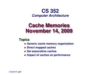
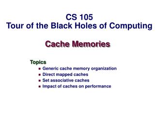
Cache MemoriesSeptember 30, 2008 15-213“The course that gives CMU its Zip!” Topics • Generic cache memory organization • Direct mapped caches • Set associative caches • Impact of caches on performance lecture-10.ppt
Announcements Exam grading done • Everyone should have gotten email with score (out of 72) • mean was 50, high was 70 • solution sample should be up on website soon • Getting your exam back • some got them in recitation • working on plan for everyone else (worst case = recitation on Monday) • If you think we made a mistake in grading • please read the syllabus for details about the process for handling it
Smaller, faster, more expensive memory caches a subset of the blocks 8 Cache: 9 14 3 Data is copied between levels in block-sized transfer units General cache mechanics 4 10 10 4 0 1 2 3 4 4 5 6 7 Memory: Larger, slower, cheaper memory is partitioned into “blocks” 8 9 10 10 11 12 13 14 15 From lecture-9.ppt
Cache Performance Metrics Miss Rate • Fraction of memory references not found in cache (misses / accesses) • 1 – hit rate • Typical numbers (in percentages): • 3-10% for L1 • can be quite small (e.g., < 1%) for L2, depending on size, etc. Hit Time • Time to deliver a line in the cache to the processor • includes time to determine whether the line is in the cache • Typical numbers: • 1-2 clock cycle for L1 • 5-20 clock cycles for L2 Miss Penalty • Additional time required because of a miss • typically 50-200 cycles for main memory (Trend: increasing!)
Lets think about those numbers Huge difference between a hit and a miss • 100X, if just L1 and main memory Would you believe 99% hits is twice as good as 97%? • Consider these numbers: cache hit time of 1 cycle miss penalty of 100 cycles So, average access time is: 97% hits: 1 cycle + 0.03 * 100 cycles =4 cycles 99% hits: 1 cycle + 0.01 * 100 cycles = 2 cycles This is why “miss rate” is used instead of “hit rate”
Many types of caches Examples • Hardware: L1 and L2 CPU caches, TLBs, … • Software: virtual memory, FS buffers, web browser caches, … Many common design issues • each cached item has a “tag” (an ID) plus contents • need a mechanism to efficiently determine whether given item is cached • combinations of indices and constraints on valid locations • on a miss, usually need to pick something to replace with the new item • called a “replacement policy” • on writes, need to either propagate change or mark item as “dirty” • write-through vs. write-back Different solutions for different caches • Lets talk about CPU caches as a concrete example…
L1 cache Hardware cache memories Cache memories are small, fast SRAM-based memories managed automatically in hardware • Hold frequently accessed blocks of main memory CPU looks first for data in L1, then in main memory Typical system structure: CPU chip register file ALU bus main memory bus interface
The tiny, very fast CPU register file has room for four 4-byte words The transfer unit between the CPU register file and the cache is a 4-byte word line 0 The small fast L1 cachehas room for two 4-word blocks line 1 The transfer unit between the cache and main memory is a 4-word block (16 bytes) block 10 a b c d ... The big slow main memory has room for many 4-word blocks block 21 p q r s ... block 30 w x y z ... Inserting an L1 Cache Between the CPU and Main Memory
The tiny, very fast CPU register file has room for four 4-byte words The transfer unit between the CPU register file and the cache is a 4-byte word line 0 The small fast L1 cachehas room for two 4-word blocks line 1 The transfer unit between the cache and main memory is a 4-word block (16 bytes) block 10 w w w w ... The big slow main memory has room for many 4-word blocks block 21 w w w w ... block 30 w w w w ... Inserting an L1 Cache Between the CPU and Main Memory
t tag bits per line B = 2b bytes per cache block 1 valid bit per line valid tag 0 1 • • • B–1 E lines per set • • • set 0: valid tag 0 1 • • • B–1 valid tag 0 1 • • • B–1 • • • S = 2s sets set 1: valid tag 0 1 • • • B–1 • • • valid tag 0 1 • • • B–1 • • • set S-1: valid tag 0 1 • • • B–1 General Organization of a Cache Cache is an array of sets Each set contains one or more lines Each line holds a block of data Cache size: C = B x E x S data bytes
t tag bits per line B = 2b bytes per cache block 1 valid bit per line valid tag 0 1 • • • B–1 E lines per set • • • set 0: valid tag 0 1 • • • B–1 valid tag 0 1 • • • B–1 • • • S = 2s sets set 1: valid tag 0 1 • • • B–1 • • • valid tag 0 1 • • • B–1 • • • set S-1: valid tag 0 1 • • • B–1 General Organization of a Cache Cache is an array of sets Each set contains one or more lines Each line holds a block of data Cache size: C = B x E x S data bytes
m-1 0 Addressing Caches Address A: b bits t bits s bits v tag 0 1 • • • B–1 set 0: • • • <tag> <set index> <block offset> v tag 0 1 • • • B–1 v tag 0 1 • • • B–1 set 1: • • • v tag 0 1 • • • B–1 • • • The word at address A is in the cache if the tag bits in one of the <valid> lines in set <set index> match <tag> The word contents begin at offset <block offset> bytes from the beginning of the block v tag 0 1 • • • B–1 set S-1: • • • v tag 0 1 • • • B–1
m-1 0 Addressing Caches Address A: b bits t bits s bits v tag 0 1 • • • B–1 set 0: • • • <tag> <set index> <block offset> v tag 0 1 • • • B–1 v tag 0 1 • • • B–1 set 1: • • • v tag 0 1 • • • B–1 • • • Locate the set based on <set index> Locate the line in the set based on <tag> Check that the line is valid Locate the data in the line based on<block offset> v tag 0 1 • • • B–1 set S-1: • • • v tag 0 1 • • • B–1
Example: Direct-Mapped Cache Simplest kind of cache, easy to build(only 1 tag compare required per access) Characterized by exactly one line per set. E=1 lines per set set 0: valid tag cache block set 1: cache block valid tag • • • set S-1: cache block valid tag Cache size: C = B x S data bytes
set 0: valid tag cache block set 1: cache block valid tag • • • set S-1: cache block valid tag Accessing Direct-Mapped Caches Set selection • Use the set index bits to determine the set of interest. selected set t bits s bits b bits 0 0 0 0 1 m-1 0 tag set index block offset
=1? (1) The valid bit must be set (2) The tag bits in the cache line must match the tag bits in the address = ? Accessing Direct-Mapped Caches Line matching and word selection • Line matching: Find a valid line in the selected set with a matching tag • Word selection: Then extract the word 0 1 2 3 4 5 6 7 selected set (i): 1 0110 b0 b1 b2 b3 If (1) and (2), then cache hit t bits s bits b bits 0110 i 100 m-1 0 tag set index block offset
0 1 2 3 4 5 6 7 1 0110 b0 b1 b2 b3 Accessing Direct-Mapped Caches Line matching and word selection • Line matching: Find a valid line in the selected set with a matching tag • Word selection: Then extract the word selected set (i): (3) If cache hit,block offset selects starting byte. t bits s bits b bits 0110 i 100 m-1 0 tag set index block offset
0 ? ? 1 1 1 1 0 0 M[8-9] M[0-1] M[0-1] 1 0 M[6-7] Direct-Mapped Cache Simulation M=16 byte addresses, B=2 bytes/block, S=4 sets, E=1 entry/set Address trace (reads): 0 [00002], 1 [00012], 7 [01112], 8 [10002], 0 [00002] t=1 s=2 b=1 x xx x miss hit miss miss miss v tag data
valid tag cache block set 0: valid tag cache block valid tag cache block set 1: valid tag cache block • • • valid tag cache block set S-1: valid tag cache block Example: Set Associative Cache Characterized by more than one line per set E=2 lines per set E-way associative cache
valid tag cache block set 0: cache block valid tag valid tag cache block set 1: cache block valid tag • • • cache block valid tag set S-1: cache block valid tag Accessing Set Associative Caches Set selection • identical to direct-mapped cache selected set t bits s bits b bits 0 0 0 1 m-1 0 tag set index block offset
=1? (1) The valid bit must be set (2) The tag bits in one of the cache lines must match the tag bits in the address = ? Accessing Set Associative Caches Line matching and word selection • must compare the tag in each valid line in the selected set. 0 1 2 3 4 5 6 7 1 1001 selected set (i): 1 0110 b0 b1 b2 b3 If (1) and (2), then cache hit t bits s bits b bits 0110 i 100 m-1 0 tag set index block offset
Accessing Set Associative Caches Line matching and word selection • Word selection is the same as in a direct mapped cache 0 1 2 3 4 5 6 7 1 1001 selected set (i): 1 0110 b0 b1 b2 b3 (3) If cache hit,block offset selects starting byte. t bits s bits b bits 0110 i 100 m-1 0 tag set index block offset
0 ? ? 1 00 M[0-1] 1 10 M[8-9] 1 01 M[6-7] 2-Way Associative Cache Simulation M=16 byte addresses, B=2 bytes/block, S=2 sets, E=2 entry/set Address trace (reads): 0 [00002], 1 [00012], 7 [01112], 8 [10002], 0 [00002] t=2 s=1 b=1 xx x x miss hit miss miss hit v tag data 0 0 0
Notice that middle bits used as index t bits s bits b bits 0 0 0 0 1 m-1 0 tag set index block offset
High-Order Bit Indexing Middle-Order Bit Indexing 4-line Cache 0000 0000 00 0001 0001 01 0010 0010 10 0011 0011 11 0100 0100 0101 0101 0110 0110 0111 0111 1000 1000 1001 1001 1010 1010 1011 1011 1100 1100 1101 1101 1110 1110 1111 1111 Why Use Middle Bits as Index? High-Order Bit Indexing • Adjacent memory lines would map to same cache entry • Poor use of spatial locality Middle-Order Bit Indexing • Consecutive memory lines map to different cache lines • Can hold S*B*E-byte region of address space in cache at one time
High-Order Bit Indexing Middle-Order Bit Indexing 4-line Cache 0000 0000 00 0001 0001 01 0010 0010 10 0011 0011 11 0100 0100 0101 0101 0110 0110 0111 0111 1000 1000 1001 1001 1010 1010 1011 1011 1100 1100 1101 1101 1110 1110 1111 1111 Why Use Middle Bits as Index? High-Order Bit Indexing • Adjacent memory lines would map to same cache entry • Poor use of spatial locality Middle-Order Bit Indexing • Consecutive memory lines map to different cache lines • Can hold S*B*E-byte region of address space in cache at one time
Sidebar: Multi-Level Caches Options: separate data and instruction caches, or a unified cache Unified L2 Cache Memory L1 d-cache Regs Processor disk L1 i-cache size: speed: $/Mbyte: line size: 200 B 3 ns 8 B 8-64 KB 3 ns 32 B 1-4MB SRAM 6 ns $100/MB 32 B 128 MB DRAM 60 ns $1.50/MB 8 KB 30 GB 8 ms $0.05/MB larger, slower, cheaper
What about writes? Multiple copies of data exist: • L1 • L2 • Main Memory • Disk What to do when we write? • Write-through • Write-back • need a dirty bit • What to do on a write-miss? What to do on a replacement? • Depends on whether it is write through or write back
Software caches are more flexible Examples • File system buffer caches, web browser caches, etc. Some design differences • Almost always fully associative • so, no placement restrictions • index structures like hash tables are common • Often use complex replacement policies • misses are very expensive when disk or network involved • worth thousands of cycles to avoid them • Not necessarily constrained to single “block” transfers • may fetch or write-back in larger units, opportunistically
Locality Example #1 Being able to look at code and get a qualitative sense of its locality is a key skill for a professional programmer Question: Does this function have good locality? int sum_array_rows(int a[M][N]) { int i, j, sum = 0; for (i = 0; i < M; i++) for (j = 0; j < N; j++) sum += a[i][j]; return sum; }
Locality Example #2 Question: Does this function have good locality? int sum_array_cols(int a[M][N]) { int i, j, sum = 0; for (j = 0; j < N; j++) for (i = 0; i < M; i++) sum += a[i][j]; return sum; }
Locality Example #3 Question: Can you permute the loops so that the function scans the 3-d array a[] with a stride-1 reference pattern (and thus has good spatial locality)? int sum_array_3d(int a[M][N][N]) { int i, j, k, sum = 0; for (i = 0; i < M; i++) for (j = 0; j < N; j++) for (k = 0; k < N; k++) sum += a[k][i][j]; return sum; }