Download
1 / 40
400 likes | 405 Views
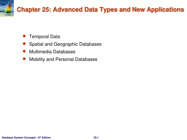
Temporal Data Spatial and Geographic Databases Multimedia Databases Mobility and Personal Databases. Chapter 25: Advanced Data Types and New Applications.

E N D
Temporal Data Spatial and Geographic Databases Multimedia Databases Mobility and Personal Databases Chapter 25: Advanced Data Types and New Applications
While most databases tend to model reality at a point in time (at the “current” time), temporal databases model the states of the real world across time. Facts in temporal relations have associated time when they are valid, which can be represented as a union of intervals. ->inputted by human The transaction time for a fact is the time interval during which the fact is current within the database system. -> recorded by system In a temporal relation, each tuple has an associated time when it is true; the time may be either valid time or transaction time. Abi-temporal relation stores both valid and transaction time. Time In Databases
Example of a temporal relation: Temporal query languages have been proposed to simplify modeling of time as well as time related queries. Time In Databases (Cont.)
date: four digits for the year (1--9999), two digits for the month (1--12), and two digits for the date (1--31). time: two digits for the hour, two digits for the minute, and two digits for the second, plus optional fractional digits. timestamp: the fields of date and time, with six fractional digits for the seconds field. Times are specified in the Universal Coordinated Time, abbreviated UTC (from the French); supports time with time zone. interval: refers to a period of time (e.g., 2 days and 5 hours), without specifying a particular time when this period starts; different from the one shown above as a pair of attributes “from” and “to”. Time Specification in SQL-92
Predicates precedes, overlaps, and contains on time intervals. Intersect can be applied on two intervals, to give a single (possibly empty) interval; the union of two intervals may or may not be a single interval. A snapshotof a temporal relation at time t consists of the tuples that are valid at time t, with the time-interval attributes projected out. Temporal selection: involves time attributes Temporal projection: the tuples in the projection inherit their time-intervals from the tuples in the original relation. Temporal join: the time-interval of a tuple in the result is the intersection of the time-intervals of the tuples from which it is derived. If intersection is empty, tuple is discarded from join. More temporal support is defined in SQL:2011. Temporal Query Languages
Spatial databases store information related to spatial locations, and support efficient storage, indexing and querying of spatial data. Special purpose index structures are important for accessing spatial data, and for processing spatial join queries. Computer Aided Design (CAD) databases store design information about how objects are constructed. E.g., designs of buildings, aircraft, layouts of integrated-circuits Geographic databases store geographic information (e.g., maps): often called geographic information systems or GIS. Spatial and Geographic Databases
Various geometric constructs can be represented in a database in a normalized fashion. Represent a line segment by the coordinates of its endpoints. Approximate a curve by partitioning it into a sequence of segments Create a list of vertices in order, or Represent each segment as a separate tuple that also carries with it the identifier of the curve (2D features such as roads). Closed polygons List of vertices in order, starting vertex is the same as the ending vertex, or Represent boundary edges as separate tuples, with each containing identifier of the polygon, or Use triangulation — divide polygon into triangles Note the polygon identifier with each of its triangles. Representation of Geometric Information
Represent design components as objects (generally geometric objects); the connections between the objects indicate how the design is structured. Simple two-dimensional objects: points, lines, triangles, rectangles, polygons. Complex two-dimensional objects: formed from simple objects via union, intersection, and difference operations. Complex three-dimensional objects: formed from simpler objects such as spheres, cylinders, and cuboids (長方體), by union, intersection, and difference operations. Design Databases
Design databases also store non-spatial information about objects (e.g., construction material, color, etc.) Spatial integrity constraints are important. E.g., pipes should not intersect, wires should not be too close to each other, etc. Representation of Geometric Constructs
Raster data consist of bit maps or pixel maps, in two or more dimensions. Example 2-D raster image: satellite image of cloud cover, where each pixel stores the cloud visibility in a particular area. Additional dimensions might include the temperature at different altitudes at different regions, or measurements taken at different points in time. Design databases generally do not store raster data. Geographic Data
Vector data are constructed from basic geometric objects: points, line segments, triangles, and other polygons in two dimensions, and cylinders, spheres, cuboids, and other polyhedrons(多角體) in three dimensions. Vector formats are often used to represent map data. Roads can be considered as two-dimensional and represented by lines and curves. Some features, such as rivers, may be represented either as complex curves or as complex polygons, depending on whether their width is relevant. Features such as regions and lakes can be depicted as polygons. Geographic Data (Cont.)
Examples of geographic data map data for vehicle navigation distribution network information for power, telephones, water supply, and sewage (下水道) Vehicle navigation systems store information about roads and services for the use of drivers: Spatial data: e.g., road/restaurant/gas-station coordinates Non-spatial data: e.g., one-way streets, speed limits, traffic congestion Global Positioning System (GPS): utilizes information broadcast from GPS satellites to find the current location of users with an accuracy of tens of meters. widely used in vehicle navigation systems Applications of Geographic Data
Nearness queries request objects that lie near a specified location. Nearest neighbor queries, given a point or an object, find the nearest object that satisfies given conditions. -> KNN query Region queries deal with spatial regions. e.g., ask for objects that lie partially or fully inside a specified region. Queries that compute intersections or unions of regions. Spatial join of two spatial relations with the location playing the role of join attributes. Spatial Queries
Spatial data are typically queried using a graphical query language; results are also displayed in a graphical manner. Graphical interfaces constitute the front-end Extensions of SQL with abstract data types, such as lines, polygons and bit maps, have been proposed to interface with back-end. allows relational databases to store and retrieve spatial information Queries can use spatial conditions (e.g., contains or overlaps). queries can mix spatial and nonspatial conditions Supported DB software: MySQL, PostGIS, Oracle Spatial, MS SQL Server, etc Spatial Queries (Cont.)
#Oracle Spatial • 使用SDO_GEOMETRY型態 • 可表示一個幾何對象,包含點、線、面、多點、多線、多面等。 • 包含的參數有: SDO_GTYPE(幾何圖形)、SDO_SRID(座標系統)、SDO_POINT、SDO_ELEM_INFO、SDO_ORDINATES(實際座標) • Example: CREATE TABLE mylake ( feature_id NUMBER PRIMARY KEY, name VARCHAR2(32), shape MDSYS.SDO_GEOMETRY); INSERT INTO mylake VALUES( 10, 'Lake Calhoun', MDSYS.SDO_GEOMETRY( 2003, NULL, NULL, (起迄皆為1,為封閉且由直線形成的多邊形,座標逆時針) MDSYS.SDO_ELEM_INFO_ARRAY(1,1003,1, 19,2003,1), MDSYS.SDO_ORDINATE_ARRAY(0,0, 10,0, 10,10, 0,10, 0,0, 4,4, 6,4, 6,6, 4,6, 4,4)) );
#Oracle Spatial(cont) • 支援R-tree和QuadTree Example:建立R-tree CREATE INDEX aa ON mylake(spape) INDEXTYPE is MDSYS. SPATIAL_INDEX; • 支援SQL Function • SDO_GEOM_SDO_INTERSECTION • SDO_GEOM_SDO_AREA • SDO_GEOM_SDO_DISTANCE • SDO_GEOM_RELATE:回傳Boolean值
k-d tree - early structure used for indexing in multiple dimensions. Each level of a k-d tree partitions the space into two. choose one dimension for partitioning at the root level of the tree. choose another dimensions for partitioning nodes at the next level and so on, cycling through the dimensions. In each node, approximately half of the points stored in the sub-tree fall on one side and half on the other. Partitioning stops when a node has less than a given maximum number of points. The k-d-B tree extends the k-d tree to allow multiple child nodes for each internal node; well-suited for secondary storage. Indexing of Spatial Data
Each line in the figure (other than the outside box) corresponds to a node in the k-d tree. The maximum number of points in a leaf node has been set to 1. The numbering of the lines in the figure indicates the level of the tree at which the corresponding node appears. Division of Space by a k-d Tree
Practice • Draw the corresponding tree structure (given node id and line position). (2.5) (1) (0.8 1.5 2.5)
s. Example of a k-d tree
Quadtrees Each node of a quadtree is associated with a rectangular region of space; the top node is associated with the entire target space. Each non-leaf nodes divides its region into four equal sized quadrants Correspondingly each such node has four child nodes corresponding to the four quadrants and so on Leaf nodes have between zero and some fixed maximum number of points (set to 1 in example). Example: Division of Space by Quadtrees
Practice • Draw the corresponding tree structure.
PR quadtree: The above type of quadtree is called a PR quadtree, to indicate that it stores points, and the space is divided based on regions, rather than on the actual set of points stored. Extensions of k-d trees and PR quadtrees have been proposed to index line segments and polygons Require splitting segments/polygons into pieces at partitioning boundaries Same segment/polygon may be represented at several leaf nodes Quadtrees (Cont.)
R-trees are a N-dimensional extension of B+-trees, useful for indexing sets of rectangles and other polygons. Supported in many modern database systems, along with variants like R+ -trees and R*-trees. Basic idea: generalize the notion of a one-dimensional interval associated with each B+ -tree node to an N-dimensional interval, that is, an N-dimensional rectangle. Will consider only the two-dimensional case (N = 2) generalization for N > 2 is straightforward, although R-trees work well only for relatively small N R-Trees
A rectangular bounding box is associated with each tree node. Bounding box of a leaf node is a minimum sized rectangle that contains all the rectangles/polygons associated with the leaf node. The bounding box associated with a non-leaf node contains the bounding box associated with all its children. Bounding box of a node serves as its key in its parent node (if any) Bounding boxes of children of a node are allowed to overlap A polygon is stored only in one node, and the bounding box of the node must contain the polygon. The storage efficiency or R-trees is better than that of k-d trees or quadtrees since a polygon is stored only once. R Trees (Cont.)
A set of rectangles (solid line) and the bounding boxes (dashed line) of the nodes of an R-tree for the rectangles. The R-tree is shown on the right. Example R-Tree
To find data items (rectangles/polygons) intersecting (overlapping) a given query point/region, do the following, starting from the root node: If the node is a leaf node, output the data items whose keys intersect the given query point/region. Else, for each child of the current node whose bounding box overlaps the query point/region, recursively search the child Can be very inefficient in worst case since multiple paths may need to be searched but works acceptably in practice. Simple extensions of search procedure to handle predicates contained-in and contains Search in R-Trees
Insertion in R-Trees • To insert a data item: • Find a leaf to store it, and add it to the leaf • To find leaf, follow a child (if any) whose bounding box contains the bounding box of the data item, else child whose overlap with data item’s bounding box is maximum • Handle overflows by splits (as in B+-trees) • Split procedure is different though (see below) • Adjust bounding boxes starting from the leaf upwards • Split procedure: • Goal: divide entries of an overfull node into two sets such that the bounding boxes have minimum total area • This is a heuristic. Alternatives like minimum overlap are possible -> R* tree • Finding the “best” split is expensive, use heuristics instead • See next slide
Splitting an R-Tree Node • Quadratic (二次方) split divides the entries in a node into two new nodes as follows • Find pair of entries with “maximum separation” • that is, the pair such that the bounding box of the two would has the maximum wasted space (area of bounding box – sum of areas of two entries) <- see the next page • Place these entries in two new nodes • Repeatedly find the entry with “maximum preference” for one of the two new nodes, and assign the entry to that node • Preference of an entry to a node is the increase in area of bounding box if the entry is added to the other node • Stop when half the entries have been added to one node • Then assign remaining entries to the other node • Cheaper linear split heuristic works in time linear in number of entries, • Cheaper but generates slightly worse splits.
Node Splitting The total area of the two covering rectangles after a split should be minimized.
Deleting in R-Trees • Deletion of an entry in an R-tree done much like a B+-tree deletion. • In case of underfull node, borrow entries from a sibling if possible, else merging sibling nodes • Alternative approach removes all entries from the underfull node, deletes the node, then reinserts all entries
To provide database functions such as indexing and consistency, it is desirable to store multimedia data in a database rather than storing them outside the database, in a file system The database must handle large object representation. Similarity-based retrieval must be provided by special index structures. Must provide guaranteed steady retrieval rates for continuous-media data. Multimedia Databases
Store and transmit multimedia data in compressed form JPEG and GIF the most widely used formats for image data. MPEG standard for video data use commonalties among a sequence of frames to achieve a greater degree of compression. MPEG-1 quality comparable to VHS video tape. stores a minute of 30-frame-per-second video and audio in approximately 12.5 MB MPEG-2 designed for digital broadcast systems and digital video disks; negligible loss of video quality. Compresses 1 minute of audio-video to approximately 17 MB. Several alternatives of audio encoding MPEG-1 Layer 3 (MP3), RealAudio, WindowsMedia format, etc. Multimedia Data Formats
Most important types are video and audio data. Characterized by high data volumes and real-time information-delivery requirements. Data must be delivered sufficiently fast that there are no gaps in the audio or video. Data must be delivered at a rate that does not cause overflow of system buffers. Synchronization among distinct data streams must be maintained Video of a person speaking must show lips moving synchronously with the audio Continuous-Media Data
Video-on-demand systems deliver video from central video servers, across a network, to terminals Must guarantee end-to-end delivery rates Current video-on-demand servers are based on file systems; existing database systems do not meet real-time response requirements. Multimedia data are stored on several disks (RAID configuration), or on tertiary(第三方) storage for less frequently accessed data. Head-end terminals - used to view multimedia data PCs or TVs attached to a small, inexpensive computer called a set-top box (機上盒). Video Servers
Examples of similarity based retrieval Pictorial data: Two pictures or images that are slightly different as represented in the database may be considered the same by a user. E.g., identify similar designs for registering a new trademark. Audio data: Speech-based user interfaces allow the user to give a command or identify a data item by speaking. E.g., test user input against stored commands. Handwritten data: Identify a handwritten data item or command stored in the database Similarity-Based Retrieval
A mobile computing environment consists of mobile computers, referred to as mobile hosts, and a wired network of computers. Mobile host may be able to communicate with wired network through a wireless digital communication network Wireless local-area networks (within a building) E.g., Avaya’s Orinico Wireless LAN Wide areas networks Cellular digital packet networks 3 G and 2.5 G cellular networks Mobile Computing Environments
Mobile Computing Environments (Cont.) • A model for mobile communication • Mobile hosts communicate to the wired network via computers referred to as mobile support (or base) stations. • Each mobile support station manages those mobile hosts within its cell. • When mobile hosts move between cells, there is a handoff of control from one mobile support station to another. • Direct communication, without going through a mobile support station is also possible between nearby mobile hosts • Supported, e.g., by the Bluetooth standard (up to 10 meters, at up to 721 kbps)
New issues for query optimization. Connection time charges and number of bytes transmitted Energy (battery power) is a scarce resource and its usage must be minimized Mobile user’s locations may be a parameter of the query GIS queries Techniques to track locations of large numbers of mobile hosts Broadcast data can enable any number of clients to receive the same data at no extra cost leads to interesting querying and data caching issues. Users may need to be able to perform database updates even while the mobile computer is disconnected. E.g., mobile salesman records sale of products on (local copy of) database. Can result in conflicts detected on reconnection, which may need to be resolved manually. Database Issues in Mobile Computing