Machine Learning

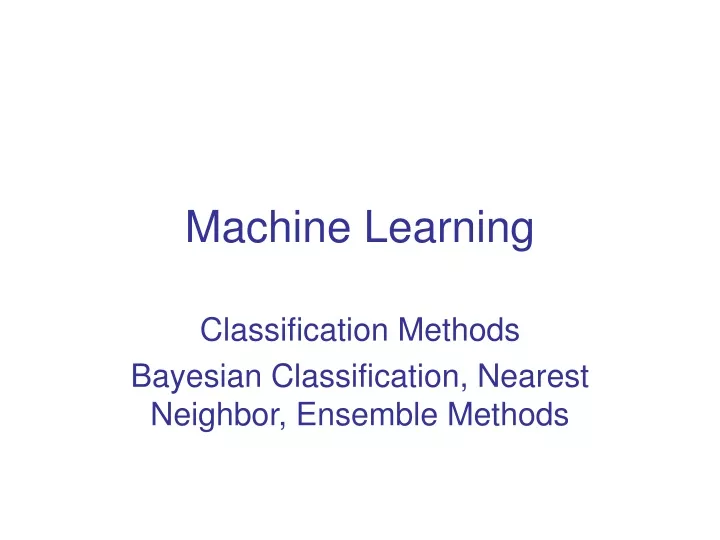
Machine Learning Classification Methods Bayesian Classification, Nearest Neighbor, Ensemble Methods

Bayesian Classification: Why? A statistical classifier: performs probabilistic prediction, i.e., predicts class membership probabilities Foundation: Based on Bayes’ Theorem. Performance: A simple Bayesian classifier, naïve Bayesian classifier, has comparable performance with decision tree and selected neural network classifiers Incremental: Each training example can incrementally increase/decrease the probability that a hypothesis is correct — prior knowledge can be combined with observed data January 1, 2020 Data Mining: Concepts and Techniques 2

Bayes’ Rule Who is who in Bayes’ rule

Example of Bayes Theorem • Given: • A doctor knows that meningitis causes stiff neck 50% of the time • Prior probability of any patient having meningitis is 1/50,000 • Prior probability of any patient having stiff neck is 1/20 • If a patient has stiff neck, what’s the probability he/she has meningitis?

Choosing Hypotheses • Maximum Likelihood hypothesis: • Generally we want the most probable hypothesis given training data.This is the maximum a posteriori hypothesis: • Useful observation: it does not depend on the denominator P(d)

Bayesian Classifiers • Consider each attribute and class label as random variables • Given a record with attributes (A1, A2,…,An) • Goal is to predict class C • Specifically, we want to find the value of C that maximizes P(C| A1, A2,…,An ) • Can we estimate P(C| A1, A2,…,An ) directly from data?

Bayesian Classifiers • Approach: • compute the posterior probability P(C | A1, A2, …, An) for all values of C using the Bayes theorem • Choose value of C that maximizes P(C | A1, A2, …, An) • Equivalent to choosing value of C that maximizes P(A1, A2, …, An|C) P(C) • How to estimate P(A1, A2, …, An | C )?

Naïve Bayes Classifier • Assume independence among attributes Ai when class is given: • P(A1, A2, …, An |C) = P(A1| Cj) P(A2| Cj)… P(An| Cj) • Can estimate P(Ai| Cj) for all Ai and Cj. • This is a simplifying assumption which may be violated in reality • The Bayesian classifier that uses the Naïve Bayes assumption and computes the MAP hypothesis is called Naïve Bayes classifier

How to Estimate Probabilities from Data? • For continuous attributes: • Discretize the range into bins • one ordinal attribute per bin • violates independence assumption • Two-way split: (A < v) or (A > v) • choose only one of the two splits as new attribute • Probability density estimation: • Assume attribute follows a normal distribution • Use data to estimate parameters of distribution (e.g., mean and standard deviation) • Once probability distribution is known, can use it to estimate the conditional probability P(Ai|c)

How to Estimate Probabilities from Data? • Normal distribution: • One for each (Ai,ci) pair • For (Income, Class=No): • If Class=No • sample mean = 110 • sample variance = 2975

Naïve Bayesian Classifier: Training Dataset Class: C1:buys_computer = ‘yes’ C2:buys_computer = ‘no’ New Data: X = (age <=30, Income = medium, Student = yes Credit_rating = Fair) January 1, 2020 Data Mining: Concepts and Techniques 12

Naïve Bayesian Classifier: An Example Given X (age=youth, income=medium, student=yes, credit=fair) Maximize P(X|Ci)P(Ci), for i=1,2 First step: Compute P(C) The prior probability of each class can becomputed based on the training tuples: P(buys_computer=yes)=9/14=0.643 P(buys_computer=no)=5/14=0.357

Naïve Bayesian Classifier: An Example Given X (age=youth, income=medium, student=yes, credit=fair) Maximize P(X|Ci)P(Ci), for i=1,2 Second step: compute P(X|Ci) P(X|buys_computer=yes)= P(age=youth|buys_computer=yes)x P(income=medium|buys_computer=yes) x P(student=yes|buys_computer=yes)x P(credit_rating=fair|buys_computer=yes) = 0.044 P(age=youth|buys_computer=yes)=0.222 P(income=medium|buys_computer=yes)=0.444 P(student=yes|buys_computer=yes)=6/9=0.667 P(credit_rating=fair|buys_computer=yes)=6/9=0.667

Naïve Bayesian Classifier: An Example Given X (age=youth, income=medium, student=yes, credit=fair) Maximize P(X|Ci)P(Ci), for i=1,2 Second step: compute P(X|Ci) P(X|buys_computer=no)= P(age=youth|buys_computer=no)x P(income=medium|buys_computer=no) x P(student=yes|buys_computer=no) x P(credit_rating=fair|buys_computer=no) = 0.019 P(age=youth|buys_computer=no)=3/5=0.666 P(income=medium|buys_computer=no)=2/5=0.400 P(student=yes|buys_computer=no)=1/5=0.200 P(credit_rating=fair|buys_computer=no)=2/5=0.400

Naïve Bayesian Classifier: An Example Given X (age=youth, income=medium, student=yes, credit=fair) Maximize P(X|Ci)P(Ci), for i=1,2 We have computed in the first and second steps: P(buys_computer=yes)=9/14=0.643 P(buys_computer=no)=5/14=0.357 P(X|buys_computer=yes)= 0.044 P(X|buys_computer=no)= 0.019 Third step: compute P(X|Ci)P(Ci) for each class P(X|buys_computer=yes)P(buys_computer=yes)=0.044 x 0.643=0.028 P(X|buys_computer=no)P(buys_computer=no)=0.019 x 0.357=0.007 The naïve Bayesian Classifier predicts X belongs to class (“buys_computer = yes”)

Example Training set : (Öğrenme Kümesi) k Given a Test Record:

Avoiding the 0-Probability Problem • If one of the conditional probability is zero, then the entire expression becomes zero • Probability estimation: c: number of classes p: prior probability m: parameter

Naïve Bayes (Summary) • Advantage • Robust to isolated noise points • Handle missing values by ignoring the instance during probability estimate calculations • Robust to irrelevant attributes • Disadvantage • Assumption: class conditional independence, which may cause loss of accuracy • Independence assumption may not hold for some attribute. Practically, dependencies exist among variables • Use other techniques such as Bayesian Belief Networks (BBN)

Remember • Bayes’ rule can be turned into a classifier • Maximum A Posteriori (MAP) hypothesis estimation incorporates prior knowledge; Max Likelihood (ML) doesn’t • Naive Bayes Classifier is a simple but effective Bayesian classifier for vector data (i.e. data with several attributes) that assumes that attributes are independent given the class. • Bayesian classification is a generative approach to classification

Classification Paradigms • In fact, we can categorize three fundamental approaches to classification: • Generative models: Model p(x|Ck) and P(Ck) separately and use the Bayes theorem to find the posterior probabilities P(Ck|x) • E.g. Naive Bayes, Gaussian Mixture Models, Hidden Markov Models,… • Discriminative models: • Determine P(Ck|x) directly and use in decision • E.g. Linear discriminant analysis, SVMs, NNs,… • Find a discriminant function f that maps x onto a class label directly without calculating probabilities Slide from B.Yanik

Bayesian Belief Networks Bayesian belief network allows a subset of the variables to be conditionally independent A graphical model of causal relationships (neden sonuç ilişkilerini simgeleyen bir çizge tabanlı model) Represents dependency among the variables Gives a specification of joint probability distribution X Y Z P • Nodes: random variables • Links: dependency • X and Y are the parents of Z, and Y is the parent of P • No dependency between Z and P • Has no loops or cycles January 1, 2020 Data Mining: Concepts and Techniques 23

Bayesian Belief Network: An Example (FH, S) (FH, ~S) (~FH, S) (~FH, ~S) LC 0.8 0.7 0.5 0.1 ~LC 0.2 0.5 0.3 0.9 Family History Smoker The conditional probability table (CPT) for variable LungCancer: LungCancer Emphysema CPT shows the conditional probability for each possible combination of its parents Derivation of the probability of a particular combination of values of X, from CPT: PositiveXRay Dyspnea Bayesian Belief Networks January 1, 2020 Data Mining: Concepts and Techniques 24

Training Bayesian Networks Several scenarios: Given both the network structure and all variables observable: learn only the CPTs Network structure known, some hidden variables: gradient descent (greedy hill-climbing) method, analogous to neural network learning Network structure unknown, all variables observable: search through the model space to reconstruct network topology Unknown structure, all hidden variables: No good algorithms known for this purpose Ref. D. Heckerman: Bayesian networks for data mining January 1, 2020 Data Mining: Concepts and Techniques 25

Lazy Learners • The classification algorithms presented before are eager learners • Construct a model before receiving new tuples to classify • Learned models are ready and eager to classify previously unseen tuples • Lazy learners • The learner waits till the last minute before doing any model construction • In order to classify a given test tuple • Store training tuples • Wait for test tuples • Perform generalization based on similarity between test and the stored training tuples

Lazy vs Eager

Basic k-Nearest Neighbor Classification • Given training data • Define a distance metric between points in input space D(x1,xi) • E.g., Eucledian distance, Weighted Eucledian, Mahalanobis distance, TFIDF, etc. • Training method: • Save the training examples • At prediction time: • Find the ktraining examples (x1,y1),…(xk,yk) that are closest to the test example x given the distance D(x1,xi) • Predict the most frequent class among those yi’s.

Nearest-Neighbor Classifiers • Requires three things • The set of stored records • Distance Metric to compute distance between records • The value of k, the number of nearest neighbors to retrieve • To classify an unknown record: • Compute distance to other training records • Identify k nearest neighbors • Use class labels of nearest neighbors to determine the class label of unknown record (e.g., by taking majority vote)

K-Nearest Neighbor Model Classification: Regression:

K-Nearest Neighbor Model: Weighted by Distance Classification: Regression: 31

Definition of Nearest Neighbor K-nearest neighbors of a record x are data points that have the k smallest distance to x

Voronoi Diagram Decision surface formed by the training examples • Each line segment is equidistance between points in opposite classes. • The more points, the more complex the boundaries.

The decision boundary implemented by 3NN The boundary is always the perpendicular bisector of the line between two points (Voronoi tessellation) Slide by Hinton

Nearest Neighbor Classification… • Choosing the value of k: • If k is too small, sensitive to noise points • If k is too large, neighborhood may include points from other classes

Determining the value of k • In typical applications k is in units or tens rather than in hundreds or thousands • Higher values of k provide smoothing that reduces the risk of overfitting due to noise in the training data • Value of k can be chosen based on error rate measures • We should also avoid over-smoothing by choosing k=n, where n is the total number of tuples in the training data set

Determining the value of k Given training examples Use N fold cross validation Search over K = (1,2,3,…,Kmax). Choose search size Kmax based on compute constraints Calculated the average error for each K: Calculate predicted class for each training point (using all other points to build the model) Average over all training examples Pick K to minimize the cross validation error

Example Example from J. Gamper

Choosing k Slide from J. Gamper

Nearest neighbor Classification… • k-NN classifiers are lazy learners • It does not build models explicitly • Unlike eager learners such as decision tree induction and rule-based systems • Adv: No training time • Disadv: • Testing time can be long, classifying unknown records are relatively expensive • Curse of Dimensionality : Can be easily fooled in high dimensional spaces • Dimensionality reduction techniques are often used

Ensemble Methods • One of the eager methods => builds model over the training set • Construct a set of classifiers from the training data • Predict class label of previously unseen records by aggregating predictions made by multiple classifiers

General Idea

Why does it work? • Suppose there are 25 base classifiers • Each classifier has error rate,  = 0.35 • Assume classifiers are independent • Probability that the ensemble classifier makes a wrong prediction:

Examples of Ensemble Methods • How to generate an ensemble of classifiers? • Bagging • Boosting • Random Forests

Bagging: Bootstrap AGGregatING • Bootstrap: data resampling • Generate multiple training sets • Resample the original training data • With replacement • Data sets have different “specious” patterns • Sampling with replacement • Each sample has probability (1 – 1/n)n of being selected • Build classifier on each bootstrap sample • Specious patterns will not correlate • Underlying true pattern will be common to many • Combine the classifiers: Label new test examples by a majority vote among classifiers

Boosting • An iterative procedure to adaptively change distribution of training data by focusing more on previously misclassified records • Initially, all N records are assigned equal weights • Unlike bagging, weights may change at the end of boosting round • The final classifier is the weighted combination of the weak classifiers.

Boosting • Records that are wrongly classified will have their weights increased • Records that are classified correctly will have their weights decreased • Example 4 is hard to classify • Its weight is increased, therefore it is more likely to be chosen again in subsequent rounds

Example: AdaBoost • Base classifiers (weak learners): C1, C2, …, CT • Error rate: • Importance of a classifier:

Example: AdaBoost • Weight update: • If any intermediate rounds produce error rate higher than 50%, the weights are reverted back to 1/n and the resampling procedure is repeated • Classification:

Machine Learning