Download
1 / 27
270 likes | 273 Views
Learn about the concepts of covariance and correlation in business analytics, and how they can be used to analyze relationships between variables. Explore examples such as predicting election results and analyzing bad debt patterns.

E N D
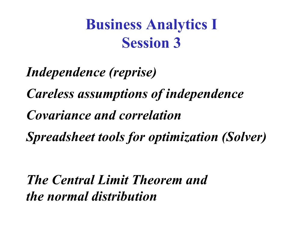
Business Analytics ISession 3 Independence (reprise) Careless assumptions of independence Covariance and correlation Spreadsheet tools for optimization (Solver) The Central Limit Theorem and the normal distribution
Predicting the Results of the 2012 U.S. Presidential Election See InTrade-2012.xls.
“Bad Debt” patterns • Did you notice any patterns in the Bad Debt data? • The 200 transactions that became bad debts averaged $7,443 per invoice. • The 9800 that were eventually paid averaged only $4,332 per invoice. • What was the effect of separating the data for small/large transactions? • The 4,533 “small”(sub-$4000) invoices that were eventually paid were paid off, on average, in about 94 days. The “large” invoices took, on average, about 10 days longer. • More strikingly, the 9,679 paid-off invoices below $9000 were paid, on average, in a bit less than 97 days … and the 121 above $9000 averaged more than 298 days to payment. Generally, how might we measure the probabilistic linkage between random variables? For example, how might we assess whether they tend to be “large” together, and “small” together?
Dependence and Covariance If two random variables are not independent, do they tend to be large together (and small together)? Or when one is large, is the other typically small (and vice versa)? Definition: The covariance of random variables X and Y is Cov(X,Y) = E[ (X–E[X]) · (Y–E[Y]) ] = E[XY]– E[X]·E[Y] . (The two expressions are algebraically the same.) A positive covariance corresponds to “typically big together, and small together.” A negative covariance corresponds to “typically, when one is big, the other is small.” Independent random variables have a covariance of 0. Emphatically: A covariance of 0 does NOT imply independence.
Correlation It is easier to interpret covariance after a rescaling: The correlation of two random variables is Corr(X,Y) = Cov(X,Y) / (StDev(X)·StDev(Y)) . Just as we use both variance (for calculations) and standard deviation (for interpretation), we use covariance (for calculations) and correlation (for interpretation). Specifically, the correlation between two random variables is a dimensionless measure of the strength of the linear relationship between those two variables. It takes values between -1 and 1.
Correlation ... beware
Definition The correlation between two random variables is a dimensionless number between 1 and -1.
Interpretation Correlation measures the strength of the linear relationship between two variables. • Strength • not the slope • Linear • misses nonlinearities completely • Two • shows only “shadows” of multidimensional relationships
A correlation of +1 would arise only if all of the points lined up perfectly. Stretching the diagram horizontally or vertically would change the perceived slope, but not the correlation.
A positive correlation signals that large values of one variable are typically associated with large values of the other. Correlation measures the “tightness” of the clustering about a single line.
A negative correlation signals that large values of one variable are typically associated with small values of the other.
But a correlation of 0 most certainly does not imply independence. Indeed, correlations can completely miss nonlinear relationships.
Back to Bad Debt Consider the data provided in the Bad Debt homework exercise. • Restrict attention to the invoices that were paid (98% of data). Let I = Invoice amount and D = days to pay. Among paid invoices, is the tendency for I and D to vary in the same or opposite direction? We can calculate E(I) and E(D) (using Excel’s =AVERAGE(range) function twice) and E(ID) (using =SUMPRODUCT(range)/COUNT(range) ). Cov(I,D) = E(ID) – E(I)·E(D) = 25636 (dollar-days) Is this a strong relationship? (Excel’s =STDEV(range) function is useful here.) Corr(I,D) = Cov(I,D) / (2463.9·93.6) = 0.111
Corr(Google searches for “Vodka”, Google searches for “SD cards”) = 0.9400 The correlation comes from common calendar peaks: a small one in June and a large one in December. Consider advertising and sales (for a seasonal product)!
The Variance of a Sum Tattoo this somewhere on your body: Var(X+Y) = Var(X) + Var(Y) + 2·Cov(X,Y) . More generally, Var(X+Y+Z) = Var(X)+Var(Y)+Var(Z) + 2·Cov(X,Y)+2·Cov(X,Z)+2·Cov(Y,Z) . and most generally, the variance of a sum is the sum of the individual variances, plus twice all of the pairwise covariances.
Portfolio Balancing See portfolios.xls
Next You are about to learn one of the handful of fundamental facts that make the universe what it is. It’s right up there with the inverse square law of gravity, Maxwell’s equations, the Theory of Relativity, the Law of Large Numbers, and the existence of the Higgs boson. It is used in every branch of science, and every functional area of management. “I know of scarcely anything so apt to impress the imagination as the wonderful form of cosmic order expressed by [what you are about to learn]. [It] would have been personified by the Greeks if they had known of it. It reigns with serenity and complete self-effacement amidst the wildest confusion. The larger the mob, the greater the apparent anarchy, the more perfect is its sway. It is the supreme law of unreason.” - Sir Francis Galton
What do these problems have in common? A firm needs to set aside funds to satisfy potential warranty claims for one product. The firm wants to minimize these funds, but also have a reasonable chance that the funds will be sufficient to cover all claims. A firm wants to keep its inventory levels down, but also limit the odds it runs out of stock in the next month. Quality control: A pharmaceutical company finds a pallet of drug vials to be 0.31kg underweight. How likely is this under normal conditions? Or when their vial injector is partly clogged? (You will see this example in OM-430) A casino offers a loss-triggered rebate to a high stakes player. They want to find the probability that they will have to pay the rebate to that customer.
What the problems had in common Each problem had these elements… • Large number of independent individual trials; • Customer purchases, warranty claims, vial weights,or gambles. • Repetition: Comparable uncertainty about each of the individual trials; • Customers indistinguishable from each other, drug vials coming from same machine, etc. • Summing: We only really care about the aggregate total outcome of these individual trials. • Total of demand, warranty claims, pallet weight, total winnings.
The Central Limit Theorem Whenever you sum a bunch of independent random variables (with comparable variances), no matter what their individual distributions may be, the result will be approximatelynormally distributed. We illustrate the probability distribution of a normally-distributed random variable through a diagram, where the total area beneath the curve is 1, and the probability of the normal variate lying in any range is the area above that range. How big is “a bunch”? Empirical studies have shown that interpreting “a bunch” as a couple of dozen or more works quite well.
The normal distribution • What you needn’t concern yourself with: • The height of the curve at any point x (a.k.a. the density function) is: • What you do need to know: • Normal distributions are completely described by their expected value and standarddeviation.
Normal distribution “rules of thumb” • P(within one standard deviation of EV) = 2/3. • P(within two standard deviations of EV) = 95%. • P(within three standard deviations of EV) = 99.7%. • P(within four standard deviations of EV) = 99.994%.
The normal distribution in Excel X • Excel commands • =NORMDIST(X, expected value, standard deviation, TRUE) • gives the probability that you get a value no higher than X • =NORMINV(probability, expected value, standard deviation) • gives the value X corresponding to the stated probability • See also: NORMSDIST, NORMSINV (when EV=0, SD=1) • Newer Excel versions: NORM.DIST, NORM.INV, etc., are identical to these commands.