Download
1 / 6
60 likes | 66 Views
Absorption design with nonlinear equilibrium. Prof. Dr. Marco Mazzotti - Institut für Verfahrenstechnik. y. y. y = m x. x. y = f(x). x. 1. Introduction to nonlinear equilibrium.

E N D
Absorption design with nonlinear equilibrium Prof. Dr. Marco Mazzotti - Institut für Verfahrenstechnik
y y y = m x x y = f(x) x 1. Introduction to nonlinear equilibrium Up to now, we always treated the case of linear equilibrium. In the linear case, the equilibrium can be described with the simple equation y = mx. However, we don’t always have such an easy relation between the gas and the liquid phase. The equilibrium relation can only be described by the general formula:
y yn+1 y = f(x) x0 x When y = mx does not apply, then Kremser`s equation is useless. However, the graphical stage-by-stage construction (and the corresponding calculation) can still be applied. Considering the initial compositions of the gas yn+1 and of the solvent x0 and the specification made for the gas outlet composition y1, we can draw in the diagram: y1
The operating line is not influenced by a nonlinear equilibrium. Therefore, the same operating line equation is still valid. The slope of the operating line depends on the solvent flow-rate L. When one of the lines is chosen as operating line, then the slope is set and thus, the required solvent flow-rate can be calculated. y yn+1 L1 /G L2 /G y = f(x) L3 /G y1 x0 x
2. Choosing an operating line There is a special operating line among the infinite number we can choose. This is the one that touches the equilibrium line at the point (xn*, yn+1). Therefore, the following equation is valid at that point: y yn+1 Lmin /G The slope corresponding to this line is the smallest possible slope, because the process cannot go beyond the equilibrium line. y = f(x) y1 x0 x The slope of this operating line can be calculated: In practice, the slope for the operating line is taken as 1 to 2 times the minimum slope:
3. Graphical construction Once the operating line is set, we can proceed with the construction seen in the linear case. The usual stage-by-stage construction is adopted, switching between equilibrium line and operating line. This gives us the number of stages, n. y yn+1 y3 3 L/G y = f(x) y2 2 y1 1 x0 x1 x2 x3 x In the beginning, we had the following unknowns: L, n and xn. The liquid flowrate L can be calculated with the slope of the operating line L/G, knowing the gas flow rate G. The number of stages n and the mole fraction xn can be read out of the graph. In our example the stage number is at least n = 3.