Download
1 / 43
430 likes | 505 Views
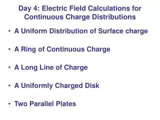
Electric Field Calculations for Line of Charge Problems. Montwood High School AP Physics C R. Casao. Electric Field Due to a Charged Rod on the Axis of the Rod. The Picture!. Divide the length of the rod L into small pieces of length dx .

E N D
Electric Field Calculations for Line of Charge Problems Montwood High School AP Physics C R. Casao
Divide the length of the rod L into small pieces of length dx. • This also divides the total charge Q on the rod into small elements of charge dq. • Over the length L of the rod, the charge on each small piece of length dx is dq. • The charge density on the rod is: • Because the charge is uniformly distributed over the length of the rod, we can set up a proportion relating the total charge per unit length to the charge per unit length for each small piece of the rod.
Each piece of length dx contains a charge dq and can be considered to be a point charge. • Each element of charge dq contributes to the net electric field E at point P. • Since the charge on the rod is positive, the net electric field at point P is directed along the negative x-axis from point P. • The distance from point P to each piece dx is x. • Electric field equation for a point charge:
The electric field contribution from each element of charge dq is designated dE. • To determine the total electric field E at point P, add the electric field contribution from each element of charge dq from the left end of the rod to the right end of the rod. • Integrate from a at the left end of the rod to (a + L) at the right end of the rod. In other words, the electric field contributions begin at a and end at (a + L). • This means that dq needs to be expressed in terms of dx because we will integrate along the x-axis from a to (a + L).
For each point charge dq: • Integrate both sides of the equation.
The integral of 1·dE is E. • For the other side of the integration, any constants can come out in front of the integral:
Substitute the (a + L) and the a into the -1/x part of the equation. The equation is: upper limit expression – lower limit expression. • Common denominator is a∙(a + L):
The Picture! • Charge per unit length:
Divide the length of the rod L into small pieces of length dx. • This also divides the total charge Q on the rod into small elements of charge dq. • Over the length L of the rod, the charge on each small piece of length dx is dq. • The charge density on the rod is:
Because the charge is uniformly distributed over the length of the rod, we can set up a proportion relating the total charge per unit length to the charge per unit length for each small piece of the rod. • Each piece of length dx contains a charge dq and can be considered to be a point charge. • Each element of charge dq contributes to the net electric field E at point P. • The total electric field E at point P is the sum of the electric fields produced by each element of charge dq from –x to x.
The electric field vector at point P for each element of charge dq can be resolved into an x component (Ex)and a y component (Ey). • At point P, the Ex components of the electric field produced by each symmetric –x and +x pair will be equal in magnitude but opposite in direction, therefore, these components cancel each other. • At point P, the net electric field will be the sum of the Ey components of the electric field produced by each element of charge dq from –x to x.
For each element of charge dq from –x to x, the values of E, r, and q all change as x changes. The relationships between these variables must be determined.
The electric field contribution from each element of charge dq is designated dEy. • To determine the total electric field E at point P, add the Ey contribution from each element of charge dq from the left end of the rod to the right end of the rod.
Integrate from -x at the left end of the rod to +x at the right end of the rod. In other words, the electric field contributions begin at -x and end at +x. • This means that dq needs to be expressed in terms of dx because we will integrate from –x to +x.
However, the radius r changes too and can be expressed in terms of x (in other words, r changes as x changes). • Integrate both sides of the equation from –x to x:
Pull the constants k, l, and y out in front of the integral sign and integrate. The y2 term cannot be removed from the integration because it is being added to the x2 term.
From a table of integration (#98): • Replacing this in the equation:
Substitute the limits of integration into the equation; remember that the equation is: upper limit expression – lower limit expression.
In this example, x is equal to 0.5·L as long as the center of the line of charge is at the origin.
MIT Visualizations • URL: http://web.mit.edu/8.02t/www/802TEAL3D/visualizations/electrostatics/index.htm • Integrating Along a Line of Charge • The Line of Charge
Consider a plastic rod having a uniformly distributed charge –Q that is bent into a circular arc of radius r. • The x-axis passes through the center of the circular arc and the point P lies at the center of curvature of the circular arc. • We will determine the electric field E due to the charged rod at point P. • The equation for arc length is: s = r·. • Divide the circular arc into small, equal pieces of length ds.
Each length ds will contain an equal amount of charge dq. • Uniform charge density allows us to set up a proportional relationship between Q, s, dq, and ds:
Each length ds containing charge dq contributes to the net electric field at point P and can be considered as a point charge: • The direction of E is towards the circular arc because the charge dq is negative. • For each symmetric length ds, the Ey component of E are equal in magnitude and opposite in direction and cancel out.
The net electric field at point P is the sum of the Ex components for each length ds from one end of the circular arc to the other end.
r is constant for every length ds along the length of the circular arc. • Each different length ds will have a different angle between the vector E and the vector Ex. • The dEx equation has two variables that change, and s, therefore, we must express one variable in terms of the other.
From the arc length equation: s = r· • Remember that r is constant, so as s changes so does . s = r· becomes ds = r·d • d represents the angle at point P for a particular length ds.
To determine the net electric field at point P, integrate from the lower end of the rod –q to the upper end of the rod +q.
Left side of integral: • Right side of integral: pull the constants k, , and r out in front of the integral
Combining the constants and the result of the integral: • Be sure to express the angle q in the correct mode on your calculator (degrees or radians).
Keep in mind that the circular arc is going to have a total length s that is some part of the circumference of a circle (C = 2·p·r). Exactly how much of a circle this is will be determined by the angles given. • Should the circular arc begin at 0° and end at 180° (or from 0 rad to prad), substitution into the sin function will give you an answer of 0 N/C for the electric field. • In that case, integrate from 0° to 90° (or 0 rad to p/2 rad) and multiply this by 2 since each half of the circular arc will contribute equally to the net electric field at point P.
If given a problem in which you have a two oppositely charged circular arcs (one from 0° to 180° and the other from 180° to 360°) arranged to form a ring of charge, you can determine the electric field of one-fourth of the circular arc and multiply the answer by 4 since each quarter will contribute equally to the net electric field at the point P. • Substituting the angles above into the sin function results in an answer of 0 N/C for the electric field.
Circular Arcs Within a Quadrant • When a circular arc lies entirely within one quadrant, write equations for the Ex component and the Ey component of the electric field contribution for each element of charge dq along the length of the circular arc. • There is no cancellation of components for a circular arc within the single quadrant.
Once you have the Ex component and the Ey component, apply the Pythagorean theorem with the two components to determine the magnitude of the resultant electric field vector. • Use a trig function (sin, cos, or tan) to determine the direction of the resultant electric field vector.