Statistics – Understanding your findings

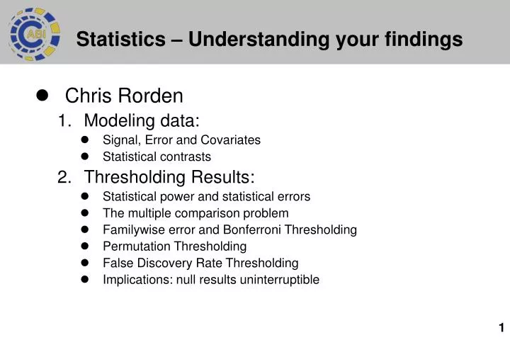
1. Statistics – Understanding your findings • Chris Rorden • Modeling data: • Signal, Error and Covariates • Statistical contrasts • Thresholding Results: • Statistical power and statistical errors • The multiple comparison problem • Familywise error and Bonferroni Thresholding • Permutation Thresholding • False Discovery Rate Thresholding • Implications: null results uninterruptible

2. The fMRI signal • Last lecture: we predict areas that are involved with a task will become brighter (after a delay) • Consider a 12-sec on, 12-sec rest task. • Our expected (model) signal should look like this:

3. Calculating statistics • Strong predictor: model predicts virtually all the variability in the observed data. • Mediocre predictor: weaker correlation between model and observed data.

4. Calculating statistics • Does our model reliably explain observed data? • Top: model good predictor (strong signal, little noise) • Middle: mediocre predictor (strong signal, lots of noise) • Bottom: mediocre predictor (little signal, little noise) • Statistical probability is based on ratio of effect amplitude divided by error (signal/noise).

5. General Linear Model • The observed data is composed of a signal that is predicted by our model and unexplained noise (Boynton et al., 1996). Design Model Amplitude (solve for) Measured Data Noise

6. What is your design model? • Model is predicted effect. • Consider Block design experiment: • Three conditions, each for 11.2sec • Press left index finger when you seeç • Press right index finger when you seeè • Do nothing when you seeé Intensity Time

7. FSL/SPM display of model • Analysis programs display model as grid. • Each column is a regressor • e.g. left / right arrows. • Each row is a volume of data • for within-subject fMRI = time • Brightness of row is model’s predicted intensity. Time Intensity Time

8. Statistical Contrasts • fMRI inference based on contrast. • Consider study with left arrow and right arrow as regressors • [1 0] identifies activation correlated with left arrows: we could expect visual and motor effects. • [1 –1] identifies regions that show more response to left arrows than right arrows. Visual effects should be similar, so should selectively identify contralateral motor cortex. • Choice of contrast crucial to inference.

9. Statistical Contrasts • t-Test is one tailed, F-test is two-tailed. • T-test: [1 –1] mutually exclusive of [-1 1]: left>right vs right>left. • F-test: [1 –1] = [-1 1]: difference between left and right. • Choice of test crucial to inference.

10. How many regressors? • We collected data during a block design, where the participant completed 3 tasks • Left hand movement • Right hand movement • Rest • We are only interested in the brain areas involved with Left hand movement. • Should we include uninteresting right hand movement as a regressor in our statistical model? • I.E. Is a [1] analysis the same as a [1 0]? • Is a [1 0] analysis identical, better, worse or different from a [1] analysis? =?

11. Meaningful regressors decrease noise • Meaningful regressors can explain some of the variability. • Adding a meaningful regressor can reduce the unexplained noise from our contrast.

12. Weight Height Explained VarianceUnexplained Variance t= Single factor… • Consider a test to see how well height predicts weight. Small t-score height only weakly predicts weight High t-score height strongly predicts weight

13. Adding a second factor… • How does an additional factor influence our test? • E.G. We can add waist diameter as a regressor. • Does this regressor influence the t-test regarding how well height predicts weight? • Consider ratio of cyan to green. Weight Height Waist Increased t Waist explains portion of weight not predicted by height. Decreased t Waist explains portion of weight predicted by height.

14. Regressors and statistics • Our analysis identifies three classes of variability: • Signal: Predicted effect of interest • Noise (aka Error): Unexplained variance • Covariates: Predicted effects that are not relevant. • E.G. Regressors with a weight of zero • Statistical significance is the ratio: • Covariates will • Improve sensitivity if they reduce error (explain otherwise unexplained variance). • Reduce sensitivity if they reduce signal (explain variance that is also predicted by our effect of interest). SignalNoise t=

15. Correlated regressors decrease signal • If a regressor is strongly correlated with our effect, it can reduce the residual signal • Our signal is excluded as the regressor explains this variability. • Example: responses highly correlated to visual stimuli

16. Summary • Regressors should be orthogonal • Each regressor describes independent variance. • Variance should not be explained by more than one regressor. • E.G. we will see that including temporal derivatives as regressors tend to help event related designs (temporal processing lecture).

17. Inferring effect size from probability maps • The claim “the parietal is more active than the frontal lobe” may be wrong • Statistical significance is based on amplitude relative to error. • Instead “the trend is for the parietal activity to be more reliable than in the frontal lobe.” • If you want to infer effect size, examine percent signal change, not statistical significance.

18. 50% 50% hematocrit hematocrit 30% 30% Statistical thresholding • E.G. erythropoietin (EPO) doping in athletes • In endurance athletes, EPO improves performance ~ 10% • Races often won by less than 1% • Without testing, athletes forced to dope to be competitive • Dangers: Carcinogenic and can cause heart-attacks • Therefore: Measure hematocrit level to identify drug users. • Problem hematocrit levels vary even in people who are not doping. If we set the threshold too high, we will fail to detect dopers (high rate of misses). If we set the threshold too low, we will accuse innocent people (high rate of false alarms).

19. Alpha level  • Statistics allow us to estimate our confidence. •  is our statistical threshold: it measures our chance of Type I error. • An alpha level of 5% means only 1/20 chance of false alarm (we will only accept p < 0.05). • An alpha level of 1% means only 1/100 chance of false alarm (p< 0.01). • Therefore, a 1% alpha is more conservative than a 5% alpha.

20. Errors • With noisy data, we will make mistakes. • Statistics allows us to • Estimate our confidence • Bias the type of mistake we make (e.g. we can decide whether we will tend to make false alarms or misses) • We can be liberal: avoiding misses • We can be conservative: avoiding false alarms. • We want liberal tests for airport weapons detection (X-ray often leads to innocent baggage being opened). • Our society wants conservative tests for criminal conviction: avoid sending innocent people to jail.

21. Reality Ho true Ho false Reject Ho Type I error false alarm Hit Decision Accept Ho Correct rejection Type II error miss Statistical Power • Statistical Power is our probability of making a Hit. • It reflects our ability to detect real effects. • To make new discoveries, we need to optimize power. • There are several ways to increase power…

22. Increasing power… • Adjust statistical threshold (e.g. p < 0.05 instead of 0.01) • However, we increase the chance of a Type I error! • Increase signal/noise ratio • Increase noise: block design, higher field magnet, higher dose • Decrease noise: meaningful regressors, temporal and spatial processing (future lectures) • Increase number of observations • Scan individuals for longer, scan more individuals • Disadvantage: time and money

23. Multiple Comparisons • Assume a 1% alpha for drug testing. • An innocent athlete only has 1% chance of being accused. • Problem: 10,500 athletes in the Olympics. • If all innocent, and  = 1%, we will wrongly accuse 105 athletes (0.01*10500)! • This is the ‘multiple comparison problem’. • The gray matter volume ~900cc (900,000mm3) • Typical fMRI voxel is 3x3x3mm (27mm3) • Therefore, we will conduct >30,000 tests • With 5% alpha, we will make >1500 false alarms!

24. Multiple Comparison Problem • If we conduct 20 tests, with an  = 5%, we will on average make one false alarm (20x0.05). • If we make twenty comparisons, it is possible that we may be making 0, 1, 2 or in rare cases even more errors. • The chance we will make at least one error is given by the formula: 1- (1- )C: if we make twenty comparisons at p < .05, we have a 1-(.95) 20 = 64% chance that we are reporting at least one erroneous finding. This is our familywise error (FWE) rate.

25. Bonferroni Correction • Bonferroni Correction: controls FWE. • For example: if we conduct 10 tests, and want a 5% chance of any errors, we will adjust our threshold to be p < 0.005 (0.05/10). • Problem: Very conservative = very little chance of detecting real effects = low power.

26. Random Field Theory 5mm • We spatially smooth our data – peaks due to noise should be attenuated by neighbors. • Worsley et al, HBM 4:58-73, 1995. • RFT uses resolution elements (resels) instead of voxels. • If we smooth our data with 8mm FWHM, then resel size is 8mm. • SPM uses RFT for FWE correction: only requires statistical map, smoothness and cluster size threshold. • Euler characteristic: unsmoothed noise will have high peaks but few clusters, smoothed data will be have lower peaks but show clustering. • RFT has many unchecked assumptions (Nichols) • Works best for heavily smoothed data (x3 voxel size) 10mm 15mm Image from Nichols

27. Permutation Thresholding Group 1 Group 2 • Prediction: Label ‘Group 1’ and ‘Group 2’ mean something. • Null Hypothesis (Ho): Labels are meaningless. • If Ho true, we should get similar t-scores if we randomly scramble order.

28. Group 1 Group 2 … … Permutation Thresholding Step 1: compute 1000 random permutations of data, record maximum T-score observed for each permutation. Observed data: max T = 4.1 • Permutation 1, max T = 3.2 • Permutation 2, max T = 2.9 • Permutation 3, max T = 3.3 • Permutation 4, max T = 2.8 • Permutation 5, max T = 3.5 … • Permutation 1000, max T = 3.1 Step 2: Rank order the 1000 maximum T-scores, the 50th most significant max T is the 5% threshold. 5 T= 3.9 Max T 0 Percentile 5%

29. Permutation Thresholding • Permutation Thresholding offers the same protection against false alarms as Bonferroni. • Typically, much more powerful than Bonferroni. • Implementations include SnPM, FSL’s randomise, and my own NPM. • Disadvantage: computing 1000 permutations means it takes x1000 times longer than typical analysis! Simulation data from Nichols et al.: Permutation always optimal. Bonferroni typically conservative. Random Fields only accurate with high DF and heavily smoothed.

30. False Discovery Rate • Traditional statistics attempts to control the False Alarm rate. • ‘False Discovery Rate’ controls the ratio of false alarms to hits. • It often provides much more power than Bonferroni correction. Consider distribution of hemacrit for our population of 10000 Olympic athletes… 5% FDR: only 5% of expelled athletes are innocent. 5% Bonferroni: only a 5% chance an innocent athlete will be accused. No dopers: Z-score is standard distribution around zero Some dopers: the dopers will form a distribution with Z-scores > 0 Z-score Z-score

31. Controlling for multiple comparisons • Bonferroni correction • We will often fail to find real results. • RFT correction • Typically less conservative than Bonferroni. • Requires large DF and broad smoothing. • Permutation Thresholding • Offers same inference as Bonferroni correction. • Typically much less conservative than Bonferroni. • Computationally very slow • FDR correction (though see www.pubmed.com/18547821) • At FDR of .05, about 5% of ‘activated’ voxels will be false alarms. • If signal is only tiny proportion of data, FDR will be similar to Bonferroni.

32. Alternatives to voxelwise analysis • Conventional fMRI statistics compute one statistical comparison per voxel. • Advantage: can discover effects anywhere in brain. • Disadvantage: low statistical power due to multiple comparisons. • Small Volume Comparison: Only test a small proportion of voxels. (Still have to adjust for RFT). • Region of Interest: Pool data across anatomical region for single statistical test. • Example: how many comparisons on this slice? • voxelwise: 1600 • SVC: 57 • ROI: 1 SPM SVC ROI

33. ROI analysis • In voxelwise analysis, we conduct an independent test for every voxel • Each voxel is noisy • Huge number of tests, so severe penalty for multiple comparisons • Alternative: pool data from region of interest. • Averaging across meaningful region should reduce noise. • One test per region, so FWE adjustment less severe. • Region must be selected independently of statistical contrast! • Anatomically predefined • Defined based on previous localizer session • Selected based on combination of conditions you will contrast. M1: movement S1: sensation

34. Inference from fMRI statistics • fMRI studies have very low power. • Correction for multiple comparisons • Poor signal to noise • Variability in functional anatomy between people. • Null results impossible to interpret. (Hard to say an area is not involved with task).