Download
1 / 46
470 likes | 664 Views
Scilab Programming – No. 2. Math 15 Lecture 11 University of California, Merced. Today – Quiz #5. Course Lecture Schedule. Grading for Math 15. Projected points. +~40 extra points (by optional hw.). UC Merced. Any Questions?.

E N D
ScilabProgramming – No. 2 Math 15 Lecture 11 University of California, Merced Today – Quiz #5
Grading for Math 15 Projected points +~40 extra points (by optional hw.)
UC Merced Any Questions?
After very first Scilab Programming experience, what did you think? SCILAB
Outline • Review • for loop • Matrix Concatenations • More programming
What is a computer programming? • A computer programming is a sequence of instructions that specifies how to perform a computation. • The computation might be something mathematical, such as solving a system of equations or finding the roots of a polynomial, • but it can also be a symbolic computation, such as searching and replacing text in a document or (strangely enough) compiling a program. Basically, all computers need someone to tell them what to do!
SCILAB The best way to learn a programming: To Practice!
When does computer programming become useful? • Let’s calculate populations of A and B species at t = 156 if the population growths of A and B are following this system of equations: • given that A = 10 and B = 5 at t = 0. • We can describe this system of difference equations in terms of matrices. 9
Here: Transition Matrix Initial Conditions • Let’s use the matrix to solve this system of equations: • For t = 156, • For t = n, 10
Well… Scilab programming will make your life easy!! • The matrix approach is certainly a easy way to solve the equations. • But I need to plot (A vs. t ) and (B vs. t) between • What is the better way to do this operation? 11
Here is the example: • If you know how to program in Scilab, only 9 lines to do the job. T =[0.9 0.1; 0.1 0.9]; // Transition matrix P0=[10;5]; // Initial Conditions Pt = P0; t = [0]; for n=1:156 Pt = [Pt,T^n*P0]; t = [t,n]; end plot(t,Pt(1,:),'-o',t,Pt(2,:),'-s') 12
To understand this program T =[0.9 0.1; 0.1 0.9]; // Transition matrix P0=[10;5]; // Initial Conditions Pt = P0; t = [0]; for n=1:156 Pt = [Pt,T^n*P0]; t = [t,n]; end plot(t,Pt(1,:),'-o',t,Pt(2,:),'-s') We don’t know what operations in these green circles yet. 13
for loop statement • for loop is a programming language statement which allows code to be repeatedly executed. A for loop is classified as an iteration statement. • The Basic Structure forvariable= starting_value: increment: ending_value commands end • The loop will be executed a fixed number of times specified by (starting_value: increment: ending_value)or the number of elements in the array variable.
for loop statement – Cont. • Slightly modified version: for variable= array commands end
for loop statement– cont. --> P = 10. P = 20. P = 30. P = 40. P = 50. for i = 1:1:5 P = i * 10 end Numbers between 1 and 5 with increment of 1 Default increment is 1, so for i = 1:5 P = i * 10 end 1st Example: 16
for loop statement– cont. --> P = 0. P = 2.5 P = 5. P = 25. P = 50. P = 500. t = [0, 0.5, 1, 5, 10, 100]; for i = t P = i * 5 end The variable, i, will be assigned from the array t. 2nd Example: 17
for loop statement– cont. • Anatomy of this loop i = 2. i = 5. i = 9. i = 14. N = 5; i = 0; // Initializing a variable for var=2:N i = i + var end
Review: for loop statement • for loop is a programming language statement which allows code to be repeatedly executed. A for loop is classified as an iteration statement. • The Basic Structure forvariable= starting_value: increment: ending_value commands end • The loop will be executed a fixed number of times specified by (starting_value: increment: ending_value)or the number of elements in the array variable.
matrix operations. – Concatenation • Concatenation • Concatenation is the process of joining smaller size matrices to form bigger ones. • This is done by putting matrices as elements in the bigger matrix. A=[1 2 3]; B = [4 5 6]; C = [7;8;9] -->[A B] // to expand columns ans = 1. 2. 3. 4. 5. 6. This doesn’t mean A is equal to [A B]. In the programming, this means [A B] is assigned to A. -->A=[A B] A = 1. 2. 3. 4. 5. 6. -->A=[A B] A = 1. 2. 3. 4. 5. 6. 4. 5. 6.
Some new matrix operations. – Cont. • Concatenation • Numbers of rows for two matrices are different. Concatenation must be row/column consistent. A=[1 2 3]; B = [4 5 6]; C = [7;8;9] -->[A C] !--error 5 inconsistent column/row dimensions -->[A;B] // to expand rows ans = 1. 2. 3. 4. 5. 6. -->A=[A;B] // Expand A A = 1. 2. 3. 4. 5. 6. -->A=[A;B] A = 1. 2. 3. 4. 5. 6. 4. 5. 6. -->A=[A C] A = 1. 2. 3. 7. 4. 5. 6. 8. 4. 5. 6. 9.
Let’s dissect this program T =[0.9 0.1; 0.1 0.9]; // Transition matrix P0=[10;5]; // Initial Conditions Pt = P0; t = [0]; for n=1:156 Pt = [Pt,T^n*P0]; t = [t,n]; end plot(t,Pt(1,:),'-o',t,Pt(2,:),'-s') We don’t know what operations in these green circles yet. 22
Making arrays • Let’s read the previous program line by line: T =[0.9 0.1; 0.1 0.9]; // Transition matrix P0=[10;5]; // Initial Conditions Pt = P0; t = [0]; Make a new array, t, with one element. • Again, this doesn’t means Pt is equal to P0. But, rather, P0 is assigned to a new matrix Pt. • At this point, Matrices P0 and Pt have exactly the same elements. Pt = 10. 5. P0 = 10. 5. 23
Expanding arrays inside the for-loop. n is assigned from 1 and 156 with increment of 1 T =[0.9 0.1; 0.1 0.9]; // Transition matrix P0=[10;5]; // Initial Conditions Pt = P0; t = [0]; for n=1:156 Pt = [Pt,T^n*P0]; t = [t,n]; end • Expanding elements in the matrix, Pt. • For each loop, add an element, TnP0, to the matrix Pt. • Expanding elements in the array, t. • For each loop, add an element, n, to the array t.
What is happening? T =[0.9 0.1; 0.1 0.9]; // Transition matrix P0=[10;5]; // Initial Conditions Pt = P0; t = [0]; for n=1:156 Pt = [Pt,T^n*P0]; t = [t,n]; end Pt = 10. 5. t = 0. Pop. A Pop. B 25
One more line to understand this program: T =[0.9 0.1; 0.1 0.9]; // Transition matrix P0=[10;5]; // Initial Conditions Pt = P0; t = [0]; for n=1:156 Pt = [Pt,T^n*P0]; t = [t,n]; end plot(t,Pt(1,:),'-o',t,Pt(2,:),'-s') To generate the graph. 26
UC Merced Any Questions?
How about this population model: • Let’s calculate populations of A, B, and C insects if the population growths of A, B, C are following this system of equations: • given that A = 10, B = 0, C=0 at t = 0. • We can describe this system of difference equations in terms of matrices. 28
First: • Let’s use the matrix to solve this system of equations: 29
Here: Transition Matrix Initial Conditions • Let’s use the matrix to solve this system of equations: • For t = 0, • For t = n, 30
UC Merced Any Questions?
Here is the Scilab program for the previous example: T =[0.8 0.1 0; 0.1 0.9 0.1; 0.1 0 0.9] // Transition matrix P0 = [10;0;0] // Initial conditions. Pt=P0; t=[0]; for i=1:35 Pt=[Pt, T^i*P0]; t = [t i]; end plot(t,Pt(1,:),t,Pt(2,:),t,Pt(3,:)) 32
Here is the Scilab program for the previous example – cont. Which curve stands for Population B? 33
Let’s add a legend for the graph T =[0.8 0.1 0; 0.1 0.9 0.1; 0.1 0 0.9] // Transition matrix P0 = [10;0;0] // Initial conditions. Pt=P0; t=[0]; for i=1:35 Pt=[Pt, T^i*P0]; t = [t i]; end plot(t,Pt(1,:),t,Pt(2,:),t,Pt(3,:)) legend('A','B','C') Since the matrix Pt contains: 1st row – Population A 2nd row – Population B 3rd row – Population C Legend’s elements must be corresponded to the orders of plot command. 34
Here is the Scilab program for the previous example – cont. 35
To make a better graph: • Scilab has a menu to modify the generated graph. • First - click Edit menu and select Current axes properties.
To make a better graph – cont. • Now, Scilab opens a new window, called axes window. • There, you can add axis labels and change font sizes of the graph.
UC Merced Any Questions?
More Example • Suppose that researchers are training a group of 60 dolphins to communicate with humans. They notice that each week 20% of untrained dolphins become trained, but 10% of trained dolphins revert to untrained status. Assume that originally all 60 dolphins were untrained approximately how many will be trained and how many untrained after 10 weeks?
Here, we are interested in tracking over time two different but interconnected quantities: trained and untrained dolphins. • There are two states in this process. • Trained and Untrained. • To help clarify things, one often begins by summarizing the transitions between two states through the use of a transition diagram.
Transition Diagram of this Process 0.80 • Suppose that researchers are training a group of 60 dolphins to communicate with humans. They notice that each week 20% of untrained dolphins become trained, but 10% of trained dolphins revert to untrained status. Assume that originally all 60 dolphins were untrained approximately how many will be trained and how many untrained after 4 weeks? Untrained 0.20 Trained 0.10 0.90
Transition Diagram and Transition Matrix 0.80 Untrained 0.20 Trained 0.10 0.90 Initial conditions
UC Merced Any Questions?
Next Lecture • More Programming in Scialb • Logical expressions • if statement • Solving some more difference equations, such as 45
Well. Can I make Scilab outputs nicer? • Answer is Yes! --> Pt = 10. 5. Pt = 9.5 5.5 Pt = 9.1 5.9 Pt = 8.78 6.22 Pt = 8.524 6.476 Pt = 8.3192 6.6808 Pt = 8.15536 6.84464 Pt = 8.024288 6.975712 Pt = 7.9194304 7.0805696 Pt = 7.8355443 7.1644557 Day = 0 Pop A= 10.00 Pop B= 5.00 Day = 1 Pop A= 9.50 Pop B= 5.50 Day = 2 Pop A= 9.10 Pop B= 5.90 Day = 3 Pop A= 8.78 Pop B= 6.22 Day = 4 Pop A= 8.52 Pop B= 6.48 Day = 5 Pop A= 8.32 Pop B= 6.68 Day = 6 Pop A= 8.16 Pop B= 6.84 Day = 7 Pop A= 8.02 Pop B= 6.98 Day = 8 Pop A= 7.92 Pop B= 7.08 Day = 9 Pop A= 7.84 Pop B= 7.16 46