Download
1 / 24
240 likes | 258 Views
An Introduction to Molecular Orbital Theory. Levels of Calculation. Classical (Molecular) Mechanics quick, simple; accuracy depends on parameterization; no consideration of orbital interaction; not MO theory) Molecular Orbital Theory (Quantum Mechanics)

E N D
Levels of Calculation • Classical (Molecular) Mechanics • quick, simple; accuracy depends on parameterization; no consideration of orbital interaction; not MO theory) • Molecular Orbital Theory (Quantum Mechanics) • Ab initio molecular orbital methods...much more demanding computationally, generally more accurate. • Semi-empirical molecular orbital methods ...computationally less demanding than ab initio, possible on a pc for moderate sized molecules, but generally less accurate than ab initio, especially for energies.
Relative Computation “Cost” • Molecular mechanics...cpu time scales as square of the number of atoms... • Calculations can be performed on a compound of ~MW 300 in a few minutes on a Pentium computer, or in a few seconds on the SGI. • This means that larger molecules (even peptides) and be modeled by MM methods.
Relative Computation “Cost” • Semi-empirical and ab initio molecular orbital methods...cpu time scales as the cube (or fourth power) of the number of orbitals (called basis functions) in the basis set. • Semi-empirical calculations on ~MW 300 compound take 10 minutes on a Pentium pc, less than one minute on our SGIs, a second on a supercomputer.
Semi-Empirical Molecular Orbital Theory • Uses simplifications of the Schrödinger equation E = H to estimate the energy of a system (molecule) as a function of the geometry and electron distribution. • The simplifications require empirically derived (not theoretical) parameters (“fudge factors”) to bring calculated values in agreement with observed values, hence the term semi-empirical.
Properties Calculated by Molecular Orbital Theory • Geometry (bond lengths, angles, dihedrals) • Energy (enthalpy of formation, free energy) • Vibrational frequencies, UV-Vis spectra • NMR chemical shifts • IP, Electron affinity (Koopman’s theorem) • Atomic charge distribution (...ill defined) • Electrostatic potential (interaction w/ point +) • Dipole moment.
History of Semi-Empirical Molecular Orbital Theory • 1930’s Hückel treated systems only • 1952 Dewar PMO; first semi- quantitative application • 1960’s Hoffmann Extended Huckel; included bonds • 1965 Pople CNDO; first useful MO program • 1967 Pople INDO
History... • 1975 Dewar MINDO/3; was widely used • 1977 Dewar MNDO • 1985 Dewar AM1; added vdW attraction & H-bonding • 1989 Stewart PM3; larger training set • 1970’s Zerner ZINDO; includes transition metals, parameterized for calculating UV-Vis spectra
Basis of Molecular Orbital Theory • Schrödinger equation: E = H (can be solved exactly for the Hydrogen atom, but nothing larger) P.A.M. Dirac, 1929: “The underlying physical laws necessary for the mathematical theory of a large part of physics and the whole of chemistry are thus completely known.”
Basis of M.O. Theory... • Simplifying assumptions are employed to ‘solve’ the Schrödinger equation approximately: • Born-Oppenheimer approximation allows separate treatment of nuclei and electrons • Hartree-Fock independent electron approximation allows each electron to be considered as being affected by the sum (field) of all other electrons. • LCAO Approximation • Variational Principle
Born-Oppenheimer Approx. • States that electron motion is independent of nuclear motion, thus the energies of the two are uncoupled and can be calculated separately. • Derives from the large difference in the mass of nuclei and electrons, and the assumption that the motion of nuclei can be ignored because they move very slowly compared to electrons Htota (Tn) + Te + Vne + Vn + Ve Kinetic energy Potential energy (Tn is omitted; this ignores relativistic effects, yielding the electronic Schrödinger equation.)
Hartree-Fock Approximation • Assumes that each electron experiences all the others only as a whole (field of charge) rather than individual electron-electron interactions. • Introduces a Fock operator F: F which is the sum of the kinetic energy of an electron, a potential that one electron would experience for a fixed nucleus, and an average of the effects of the other electrons.
LCAO Approximation • Electron positions in molecular orbitals can be approximated by a Linear Combination of Atomic Orbitals. • This reduces the problem of finding the best functional form for the molecular orbitals to the much simpler one of optimizing a set of coefficients (cn) in a linear equation: • = c1f1 + c2f2 + c3f3 + c4f4 + … where is the molecular orbital wavefunction andfnrepresent atomic orbital wavefunctions.
Variational Principle • The energy calculated from any approximation of the wavefunction will be higher than the true energy. • The better the wavefunction, the lower the energy (the more closely it approximates reality). • Changes are made systematically to minimize the calculated energy. • At the energy minimum (which approximates the true energy of the system), dE = 0.
Basis sets • A basis set is a set of mathematical equations used to represent the shapes of spaces (orbitals) occupied by the electrons and their energies. • Basis sets in common use have a simple mathematical form for representing the radial distribution of electron density. • Most commonly used are Gaussian basis sets, which approximate the better, but more complicated Slater-Type orbitals (STO).
Slater-type orbitals (STO) • Slater-type orbitals describe the electron distribution fairly well, but they are not simple enough to manipulate mathematically. • Several Gaussian-type orbitals can be added to approximate the STO. Four GTO’s mimic one STO.
Basis Sets • STO-3G (Slater-type orbitals approximated by 3 Gaussian functions)…minimal basis set, commonly used in Semi-Empirical MO calculations. (L-click here)
Hartree-Fock Self-Consistent Field (SCF) Method... • Computational methodology: • guess the orbital occupation (position) of an electron • guess the potential each electron would experience from all other electrons (taken as a group) • solve for Fock operators to generate a new, improved guess at the positions of the electrons • repeat above two steps until the wavefunction for the electrons is consistent with the field that it and the other electrons produce (SCF).
Semi-empirical MO Calculations:Further Simplifications • Neglect core (1s) electrons; replace integral for Hcore by an empirical or calculated parameter • Neglect various other interactions between electrons on adjacent atoms: CNDO, INDO, MINDO/3, MNDO, etc. • Add parameters so as to make the simplified calculation give results in agreement with observables (spectra or molecular properties).
Steps in Performing a Semi-empirical M O Calculation • Construct a model or input structure from MM calculation, X-ray file, or other source (database) • optimize structure using MM method to obtain a good starting geometry • select MO method (usually AM1 or PM3) • specify charge and spin multiplicity (s = n + 1) • select single point or geometry optimization • set termination condition (time, cycles, gradient) • select keywords (from list of >100).
Comparison of Results Mean errors relative to experimental measurements MINDO/3MNDOAM1PM3 Hf, kcal/mol 11.7 6.6 5.9 -- IP, eV -- 0.69 0.52 0.58 , Debyes -- 0.33 0.24 0.28 r, Angstroms -- 0.054 0.050 0.036 degrees -- 4.3 3.3 3.9
More results... Enthalpy of Formation, kcal/mol MM3PM3Exp’t ethane -19.66 -18.14 -- propane -25.32 -23.62 -24.8 cyclopropane 12.95 16.27 12.7 cyclopentane -18.87 -23.89 -18.4 cyclohexane -29.95 -31.03 -29.5
Some Applications... • Calculation of reaction pathways (mechanisms) • Determination of reaction intermediates and transition structures • Visualization of orbital interactions (formation of new bonds, breaking bonds as a reaction proceeds) • Shapes of molecules including their charge distribution (electron density)
…more Applications • QSAR (Quantitative Structure-Activity Relationships) • CoMFA (Comparative Molecular Field Analysis) • Remote interactions (those beyond normal covalent bonding distance) • Docking (interaction of molecules, such as pharmaceuticals with biomolecules) • NMR chemical shift prediction.