Download
1 / 66
680 likes | 785 Views
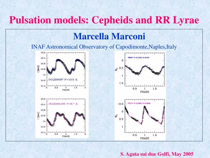
Pulsation models: Cepheids and RR Lyrae. Marcella Marconi INAF Astronomical Observatory of Capodimonte,Naples,Italy. S. Agata sui due Golfi, May 2005. Outline. What are pulsating stars ?. Why to model pulsating stars ?. Why do Cepheids and RR Lyrae pulsate

E N D
Pulsation models: Cepheids and RR Lyrae Marcella Marconi INAF Astronomical Observatory of Capodimonte,Naples,Italy S. Agata sui due Golfi, May 2005
Outline What are pulsating stars ? Why to model pulsating stars ? Why do Cepheids and RR Lyrae pulsate and why the instability strip is a strip ? What are the possible theoretical approaches to build a pulsating model ? What are the implications for the distance scale and the main uncertainties ? S. Agata sui due Golfi, May 2005
Pulsating stars Pulsating stars are intrinsic variables showing cyclic or periodic variations on a time scale which is of the order of the free fall time. In the simplest case they pulsate radially Period hours hundreds of days Mag lim. oss. a few magnitudes R/R up to ~ 0.3 for the classical ones (but even more for Miras) Among the most studied pulsating stars: • Classical Cepheids (intermediate mass He burning stars) with 1d P 100 d. • RR Lyrae (old,low mass counterpart of Classical Cepheids) with 0.3 d P 1 d. S. Agata sui due Golfi, May 2005
The instability strip S. Agata sui due Golfi, May 2005
General properties of Cepheids Classical Cepheids are intermediate mass stars (3M/M12) in the central Helium burning evolutionary phase, crossing the pulsation instability strip during the so called blue loop. Is the PL relation, in the form Mj=a+b logP universal ? If the zero point and/or the slope of this relation depends on metal abundance the adoption of a universal PL relation (calibrated on LMC Cepheids) to infer the distance to external galaxies is affected by a systematic error. Many recent observational and theoretical investigations on this topic: Madore & Freedman 1990, Kochanek et al. 1997, Kennicutt et al. 1998, Sakai et al. 2004, Romaniello et al. 2005……, Bono et al. 1999, 2002, Caputo et al. 2000, Fiorentino et al. 2002…………. The theory of stellar evolution predicts that in this evolutionary phase the mass and luminosity are related: log L/L = + logM/M + γ log Z +δ logY Cepheids are observed to pulsate with periods 1d P 100 d. Since the discovery by Miss Leavitt (1912) of a Period-Magnitude (PL) relation for the Cepheids in the SMC, they have been considered powerful primary distance indicators (see HST Key Project, lessons by B. Madore in this School). S. Agata sui due Golfi, May 2005
General properties of RR Lyrae RR Lyrae are low mass Helium burning stars, on the so called Horizontal Branch (HB) in the HR diagram They are the most abundant class of pulsating stars in the Milky Way and are found both in the field and in globular clusters. pulsation periods range from ~ 0.3 d to ~ 1.0 d pulsation amplitudes range from ~ 0.2 to ~ 1.8 mag. RR Lyrae are important tracers of chemical and dynamical properties of old stellar populations S. Agata sui due Golfi, May 2005
RRab and RRc RR Lyrae are traditionally divided into two classes: RRab with longer pulsation periods and asymmetric light curves with amplitude decreasing toward the redder colours (Fundamental mode) RRc with shorter pulsation periods and almost sinusoidal light curves (First overtone mode) S. Agata sui due Golfi, May 2005
RR Lyrae as distance indicators RR Lyrae are HB stars almost constant luminosity (apart from evolutionary effects.............) Theabsolute magnitude Mv(RR) depends on metal abundance: Mv(RR) = a + b [Fe/H] An accurate knowledge Mv(RR) provides fundamental constraints to the distance to the galactic center, globular clusters, nearby galaxies... see lessons by V. Ripepi, this school S. Agata sui due Golfi, May 2005
The time scale of pulsation • As for an acoustic wave, the pulsation period should be of the order of the time required to propagate through the diameter of the star: ~ 2R/vs where vsis the mean over the whole star in its equilibrium state of the adiabatic sound velocity . • For a self gravitating structure in hydrostatic equilibrium, rotation, pulsation…) and no magnetic field and for which the pressure vanishes on the surface, the virial theorem can be written in the form: - = 3∫PdV = 3∫P/ dm = 3∫ vs²/dm = 3 vs²/ M vs (- / 3 M ) ½ ( / - )½(=r²dm) S. Agata sui due Golfi, May 2005
for given mass and radius, decreases as increases By replacing M=4/3R³ we obtain ~2/ (4/3 G ) = costant Period-density law For known stars 106 /o 10-9 white dwarfsred supergiants 3 s 1000 d S. Agata sui due Golfi, May 2005
Why to model pulsating stars On the basis of a simple theoretical approach P = cost but for Stephan-Boltzman law L = 4 R² Te4 P=P(L,M,Te) Period-Luminosity-Color-Mass (PLCM) relation 1) Connection to the distance scale problem ( cosmology) 2) Test of evolutionary theories ( ML relations, convection, overshooting.........) Observed P and colors constraints on L and/or M For Classical Cepheids L=L(M,Y,Z) PLC (!) projecting on the PL plane PL S. Agata sui due Golfi, May 2005
Driving mechanisms In the classical instability strip the pulsation mechanisms are expected to be connected with the position in the HR diagram phenomena related to L, Te (R) The pulsation key mechanisms are related to the ionization regions of the most abundant elements in a stellar envelope: H, He ed He +(Zhevakin 1953, 1954): • mechanism • k mechanism S. Agata sui due Golfi, May 2005
increases small increase of T energyis trapped small L variation because L T4 Energy excess during the subsequent expansion phase pulsation work mechanism The adiabatic exponent 3-1= (dlogT/dlog) decreases in the ionization regions. In a ionization region most of the released energy during the phases of contraction goes into ionization: Initial contraction phase S. Agata sui due Golfi, May 2005
k mechanism Opacity variations in the H, HeI, HeII ionization regions: (k=1/λ)k n T-s stellar interior positive n and s: opacity decreases during contraction of the stellar envelope producing heat loss ionization regionss becomes large and negative: small temperature variations cause an increase of during contraction further radiation trapping energy excess pulsation work S. Agata sui due Golfi, May 2005
mechanism: effect of T variations on L variations k mechanism: effect of k variations on L variations Both the k and mechanisms are efficient in driving the pulsation but the phenomenon is started by a stochastic fluctuation of the external layer properties (e.g. contraction) S. Agata sui due Golfi, May 2005
No pulsation pulsation Blue edge Why the instability strip has a BLUE boundary? If the model effective temperature is too high the H and He/He+ ionization regions are very external low density, small mass takes part in the pulsation driving through the k and mechanisms damping prevails no pulsation Only when the ionization regions are deep enough the mass involved in the pulsation driving mechanisms prevails pulsation S. Agata sui due Golfi, May 2005
pulsation No pulsation Red edge Why the instability strip has a RED boundary? Moving toward lower effective temperature the depth of the driving ionization regions increases and the mass taking part in the phenomenon is larger increasing pulsation efficiency But convection also becomes more efficient at lower effective temperatures k andgradientsare reduced quenching of pulsation (Baker & Kippenhahn 1965) When the quenching effect due to convection prevails pulsation is no more efficient red boundaryof the instability strip S. Agata sui due Golfi, May 2005
Mass conservation equation Momentum equation Energy equation + heat transfer equation The theory of stellar pulsation The equations of stellar pulsations are the fundamental equations of hydrodynamics and heat transfer. The lagrangian description is usually preferred better physical interpretation of equations S. Agata sui due Golfi, May 2005
Radially pulsating envelope model • Spherical simmetry: the star varies its volume and luminosity on the pulsation time scale but the shape remains spherical. • No rotation, no magnetic fields. • The core is excluded (nuclear reactions evolve on much longer time scales, pulsation mechanisms excited in the envelopes) • The envelope is divided in150-250 mass zones. S. Agata sui due Golfi, May 2005
Theoretical analysis by steps • Linear adiabatic analysis (Eddington 1918) Periods • Linear NONadiabatic analysis (Baker & Kippenhahn 1962, Cox 1963, Castor 1971, Iben 1971….)Periods, blue boundary of the instability strip(red boundary fixed with ad hoc assumptions) • NONlinear radiative analysis(Christy 1966, Stellingwerf 1974…..) Periods, amplitudes (max-min), blue boundary of the instability strip • NONlinear convective analysisPeriods, more accurate pulsation amplitudes (max-min) and lightcurve morphology, blueand red boundaries of the instability strip S. Agata sui due Golfi, May 2005
Linear adiabatic models Linear small amplitude approximation, equations are linearized Adiabatic oscillating mass elements do not gain/lose heat. S. Agata sui due Golfi, May 2005
Small amplitude linearized equations ↔ Let’s assume The linearized equations become: mass momentum energy radiative transfer S. Agata sui due Golfi, May 2005
The Linear Adiabatic Wave Equation (LAWE) By combining the time derivative of the momentum equation with the other two conservation equations we obtain: For adiabatic oscillation: If solutions have the form: The solution =0 is discarded because it corresponds to the perfectly static case S. Agata sui due Golfi, May 2005
An eigenvalue problem(Cox J. P. “Theory of Stellar Pulsation”) The LAWE is an ordinary second order differential equation solution contains two integration constants. The LAWE is a linear homogeneus equation in (if is a solution, also multiplied by a constant A is a solution) the absolute value of the pulsation amplitude is one of the two constants With the remaining integration constant we fix one of the two boundary conditions (at th center or at the surface). The other boundary condition is satisfied by varying the other available parameter, namely the angular frequency of pulsation σ Only some eigenfrequencies 0, 1,….and eigenfunctions 0, 1……satisfy the boundary conditions both at the center and at the surface. S. Agata sui due Golfi, May 2005
Results of the adiabatic analysis The fundamental mode eigenfunction 0 has no nodes in the range 0 r R, while k hask nodes in the range 0 r R. For each k we have two possibilities: (a) k is real constant amplitude pulsation k(r,t)= k(r) e ±ikt; (b) k is imaginary dynamical instability on a free fall timescale If k is real the pulsation period is Pk=2/ k Linear adiabatic models provide periods for the various pulsation modes (fundamental, first overtone, second overtone…………………….)
And for solutions of the form eiωt as Linear NONadiabatic models (- H/ m) 0 In this case we cannot neglect heat exchanges Solutions imply complex frequencies =+i increasing or decreasing pulsation amplitudes pulsation stability can be investigated The linearized full energy equation can be written in the form S. Agata sui due Golfi, May 2005
In the adiabatic case In the NONadiabatic case: Driving and damping regions in a stellar envelope For a zone gaining heat at the phase of minimum radius ∫PdV>0 driving For a zone releasing heat at the phase of minimum radius ∫PdV<0 damping S. Agata sui due Golfi, May 2005
The growth rate of pulsation is The growth rate and the blue edge If the sum of the closed cycle ∫PdV over all mass shells in the star is positive the driving regions prevail over the damping ones the stellar envelope does pulsate where W is the work done on the system by the restoring forces around a complete closed cycle and Ψis the total oscillation energy or, equivalently If η > 0 W>0, κ < 0 with a time dependence e±it.e-κt oscillations are excited If η < 0 W<0, κ > 0 oscillations are damped Transition from η < 0to η > 0 defines the BLUE EDGE where <dW/dt>W/ is the average rate (over one period) at which the restoring forces do work on the system and we have used σ=2π/Π S. Agata sui due Golfi, May 2005
Most linear models do not properly treat the coupling between convection and pulsation in the oscillating stellar envelope. The red edge of the instability strip in the linear NONadiabatic approximation Convection is either neglected (e.g Castor 1971, Stellingwerf 1975, Bono & Stellingwerf 1994) or included by means of the mixing length theory (e.g. Baker & Kippenhahn 1965, van Albada & Baker 1971, Tuggle and Iben 1973, Chiosi & Wood 1990, Saio & Gautschy 1998, Alibert et al. 1999) • Some authors adopt one-dimensional turbolent convection • models into their linear nonadiabatic codes (e.g. Yecko, Kollath • & Buchler 1998, Xiong, Cheng & Deng 1998) • red edge but a number of free parameters need to be calibrated againts observations On this basis the red edge can be evaluated only by means of some ad hoc assumptions (e.g. where the growth rate is maximum) or by displacing it at fixed ΔTe from the blue edge. S. Agata sui due Golfi, May 2005
On the basis of linear nonadiabatic RR Lyrae fundamental and first overtone models, van Albada & Baker (1971) derive the following important relations: Results of linear NONadiabatic RR Lyrae models where P0 is the fundamental mode period and P1 is the first overtone one The relation for P0implies that the parameter A=logL/Lo -0.81logM/Mo can be evaluated for RR Lyrae with measured period and Te Mass-Luminosity relation Helium content These relations connect a pulsation parameter (the period) which can be measured with high accuracy from observations, with stellar intrinsic parameters, which in turn depend on age and chemical composition S. Agata sui due Golfi, May 2005
The Petersen diagram for double mode RR Lyrae Some RR Lyrae pulsate both in the fundamental and in the first overtone mode (double mode pulsators or RRd). van Albada & Baker’s relations suggest that the plot of log(P1/P0) versus logP0 (Petersen 1973) is mainly a function of the stellar mass. • Independent estimate of the stellar mass (pulsational mass) • Comparison between pulsational and evolutionary mass • Mass discrepancy problem: pulsational masses significantly lower than the evolutionary ones (Cox, Hodson & Clancy 1983; Nemec 1985) • Settled with updated input physics and nonlinear, nonlocal time-dependent convective models (Cox 1991, 1995; Bono et al. 1996) S. Agata sui due Golfi, May 2005
Results of linear NONadiabatic Cepheid models Several authors predict the instability strip blue boundary as well as relations between the pulsation periods and the intrinsic stellar parameters (P(M,L,Te), P(M,R)) which are at the basis of the PL relation theoretical constraint on the problem of PL universality They do NOT find a signficant metallicity dependenc of predicted PL relation (e.g. Saio & Gautschy 1998, Alibert et al. 1999)) or a differential dependence with the adopted bands, but quite small when the V and I bands are adopted to correct for reddening (see Chiosi, Wood & Capitanio al. 1999)
In the nonlinear approach the fundamental equations are not linearized pulsation amplitudes can be obtained MAX→ ←MIN Nonlinear radiative models The first applications of the nonlinear analysis were purely radiative (e.g. Christy 1965, 1968, 1975; Buchler et al. 1990): convection was neglected no indication on the red edge ! Also both luminosity and velocity amplitudes predicted by these models turned out to be systematically larger than the observed ones
NONlinear convective pulsation models In order to predict all the relevant observables of pulsation, namely periods, amplitudes, complete topology of the instability strip, a nonlinear convective code is required. The crucial property of a nonlinear convective code is the modeling of the coupling between convection and pulsation in a stellar oscillating envelope. S. Agata sui due Golfi, May 2005
The treatment of convection and the prediction of the red boundary of the instability strip As first suggested by Baker & Kippenhahn (1965) the increasing efficiency of convection toward lower effective temperatures has a damping effect on the and mechanisms, restoring stability. Therefore, for an accurate evaluation of the red boundary we need to take into account the coupling between dynamical and convective velocity in the stellar envelope nonlocal time-dependent theory Several attempts in the literature (e.g. Stellingwerf 1982, Geymeyer 1993, Bono & Stellingwerf 1994, Feuchtinger 1998) S. Agata sui due Golfi, May 2005
Convective transport equation is the continuity equation in phase space: Castor-Stellingwerf approach Define Φ(x,u´,t) as the number density of convective element in phase space, where x is a space coordinate relative to the mean flow, u´ is the fluctuating part of the velocity (u=<u>+ u´) where derivatives are summed over relative coordinates and S is a source function that creates convective elements with small perturbed velocities (δu´≪ |u´|) and destroy them after having traveled a mean free path “l” S. Agata sui due Golfi, May 2005
By computing the moment of this equation with respect to (u´)², using the conservation equations and treating the flux of turbolent energy via a diffusion model with diffusivity |u´|l, one obtains the convective equation in the variable <(u´)²> = 2Et phase lag term containing the driver 0 Interaction of the convective and mean velocity fields diffusive component (convective overshoot) (Castor 1968, Stellingwerf 1982) S. Agata sui due Golfi, May 2005
Results of nonlinear convective models for Cepheids: I Radial velocity Light Extended atlas of theoretical light and radial velocity curves are produced. Bono, Castellani, Marconi 2000, ApJ There are two main ways to derive observed mean magnitudes: Magnitude averaged values, e.g. (B), (V),….: mean over the magnitude curve taken in magnitude units Intensity averaged values , e.g. <B>, <V>,….:mean intensity over the magnitude curve transformed into magnitude They differ from each other and from the static magnitudes, i.e. the values the stars would have were they not pulsating. For colors it is still more complicated: one has (B)-(V), <B-V>, <B>-<V> Once mean magnitudes and colors have been obtained from the predicted lightcurves, multiwavelength Period-Luminosity-Mass-Color relations can be obtained for each assumed chemical composition Constraints on the Mass-Luminosity relation if the period, the color and the distance are known Constraints on the DISTANCE if periods and colors are known and a M-L relation is assumed. By transforming the bolometric lightcurves into the observational bands UBVRIJK (static atmosphere models) magnitude and color curves mean (time-averaged over the pulsation cycle) magnitudes and colors. S. Agata sui due Golfi, May 2005
As metallicity increases the strip gets redder ! As Y increases from 0.28to0.31at Z=0.02, the strip gets bluer Results of nonlinear convective models for Cepheids: II The complete topology of the instability strip is obtained. This is a crucial point to evaluate the PL relation, which is obtained by evaluating the statistical magnitude of Cepheids at a given period. Nonlinear convective models by Bono, Marconi & Stellingwerf (1999, ApJS) and Fiorentino et al. (2002) predict that the instability strip is a function both of metallicity and helium abundance. S. Agata sui due Golfi, May 2005
Implications for the universality of the PL The strip in the HR diagram gets redder as metallicity increase. But, for each M and L, the effective temperature is anticorrelated with the Period (← Period-Density relation + Black body) The strip in the Mbol -logP diagram moves toward longer periods as metallicity increases. At fixed period more metallic pulsators are fainter at variance with a number of empirical tests in the literature (Kennicutt et al. 1998, Sasselov et al. 1997, Sakai et al. 2004 and references therein) S. Agata sui due Golfi, May 2005
Synthetic multiband PL relations By populating with a mass law distribution the predicted instability strip at varying metallicity we find that : optical synthetic PL depend on metallicity, appear to obey to a quadratic rather than to a linear relation and have a significant dispersion; all these effect are reduced when we move toward NIR bands. Caputo, Marconi, Musella 2000 A&A S. Agata sui due Golfi, May 2005
=0.03 =0.04 Methods to derive Cepheid distances as based on nonlinear convective pulsation models • PLC relations, if reddening is known: e.g. MV=α+βlogP+γ(B-V)0 for a given M-L relation In the B, V bands you also need to take into account metallicity • NIR PL relations (even if metallicity and reddening are poorly known) allow to drive accurate distances with an intrinsic uncertainty of the order of 0.05 mag. Optical PL relations are quite dispersed due to the intrinsic width of the instability strip and are not useful to derive direct distances to individual Cepheids (σ0.25 mag) S. Agata sui due Golfi, May 2005
If reddening is not known you need at leasttwo bands and two equations For each metallicity and assumed M-L relation, you can use two theoretical relations (PL and/or PLC) to evaluate 0andE(B-V) To use the PL(V) and PL(I) relations is the same as using the so called Wesenheit relations: e.g. MV-R (B-V)0 =α+βlogP(=V-R(B-V)- 0)for a given metallicity and M-L relation AV=R E(B-V) (extinction law) j,PLj =0 + RjE(B-V)e.g. V,PLV =0 + 3.3 E(B-V) j,PLC =0+rj,E(B-V)with rj, function of Rj and of the color term coefficient in the PLC e.g. V,PLCB =0 + (3.10- ) E(B-V )MV= + logP + (B-V) True distance modulus and reddening for the measured metal abundance. S. Agata sui due Golfi, May 2005
The extension to sovrasolar chemical compositions and to varying helium contents at fixed metallicity, suggests that the metallicity correction is more complicated. It is negligible for period shorter than 10 d, whereas for longer periods there is a change of sign around solar metallicity and a clear dependence on the ΔY/ΔZ ratio Fiorentino et al. 2002 Application to the extragalactic distance scale Applying the theoretical metal-dependent PL(I) and PLC(V,I) relations to the VI dataset of the Key Project HST galaxies Caputo et al. (2000) find a theoretical metallicity correction. The HST distances based on universal PL need to be corrected: / logZ ~ -0.27mag/dex where logZ is the metallicity difference between the observed galaxy and the LMC h0/[O/H] ~ +0.124 dex-1 where h0 = H0/H0 (Ho(KP) increases by about 5 %) This behaviour is in agreement with empirical spectroscopic results by Romaniello et al. (2005) and is confirmed by an extended updated model grid (Marconi et al. 2005 submitted) The predicted correction becomes in agreement with the empirical one by Kennicutt et al. If Y/Z 3.5
If reddening and chemical composition are not known you need three bands PL, PLC relations…. depend on metallicity and helium unknown quantities in the evaluation of Cepheid extragalactic distances are: the distance, the reddening and the chemical composition Observations in at least three filters + 3 theoretical relations discriminate the metallicity and reddening effects on distance determinations, in order to derive self consistent estimatesof mean and individual distances, reddenings and metal abundances (Caputo, Marconi, Ripepi 1999 ApJ; Caputo, Marconi, Musella,Pont 2001 A&A) The above method holds for each assumedΔY/ΔZ ratio. Independent constraints on this parameter are needed.
Comparison between predicted and observed light curves • Wood Arnold & Sebo (1997) on the basis of a nonlinear convective code (Wood 1974), simulate the light curve of the LMC bump Cepheid HV 905 • Tight constraints on the input parameters M, L, Te (M-L relation) • 0(LMC)=18.51±0.05 mag. • Bono, Castellani & Marconi 2002 reproduce the light curve of two Cepheids in the LMC from the OGLE (Udalski et al. 1999) database, with different period and light curve morphology good fit for the same 0 in the range 18.48-18.58 mag • Keller & Wood (2002) applied the same technique to 20 bump Cepheids in the LMC (Macho project) 0(LMC)=18.55±0.02 (intrinsic error of the average)
Results of nonlinear convective models for RR Lyrae(da Bono et al. 1997 A&AS, Bono et al. 1997 ApJ) By taking into account the nonlinearity of the problem and the coupling between dynamical and convective velocities, we are able to predict: • the detailed morphology of light and radial velocity curves and in turn to obtain accurate Bailey (Period-Amplitude) diagrams • the complete topology of the instability strip as a function of model parameters S. Agata sui due Golfi, May 2005
RRab RRc Theoretical atlas of RR Lyrae light curves Bono et al. 1997 ApJS
The Bailey diagram Observations Theory Bono et al. 1997 ApJS
The Instability strip Bono, Caputo, Marconi 1995 AJ