Download
1 / 18
180 likes | 185 Views
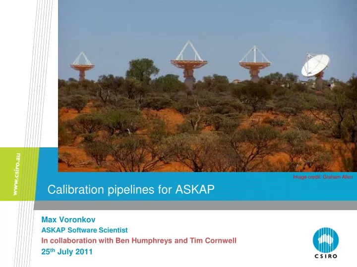
Calibration pipelines for ASKAP. Image credit: Graham Allen. Max Voronkov ASKAP Software Scientist In collaboration with Ben Humphreys and Tim Cornwell 25 th July 2011. ASKAP overview. http://www.atnf.csiro.au/projects/askap. ASKAP = Australian Square Kilometre Array Pathfinder.

E N D
Calibration pipelines for ASKAP Image credit: Graham Allen Max Voronkov ASKAP Software Scientist In collaboration with Ben Humphreys and Tim Cornwell 25th July 2011
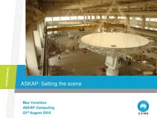
ASKAP overview http://www.atnf.csiro.au/projects/askap ASKAP = Australian Square Kilometre Array Pathfinder • Located at radio-quiet site approx. 300 km inland from Geraldton • Six antennas are already on site • Array of 36 12m antennas with phased array feeds (PAF)
ASKAP is a wide-field of view instrument Wide field of view (30 square degrees) high data rate (3 GB/s) 30 beams to fill field of view
What needs calibration? • Visibility-plane effects • Complex gain per beam per antenna • Bandpass per beam per antenna, effectively this is a complex gain per fine-resolution frequency channel (18 kHz) • Polarisation leakage per beam per antenna (per 1 MHz?) • Image-plane effects - hopefully not • Ionosphere is relatively benign at 1 GHz • Primary beam is fixed on the sky (3-axis antenna mount) • Pointing can be corrected on-the-fly, but should be fine as it is • PAF stability (synthetic beams) is still the biggest unknown. Peeling is expected to help. PAF element-based calibration is taken care of upstream. • Operations-specific calibration - not something we do in real time • Antenna positions on the ground (baseline calibration) • Global pointing model (might be done per-antenna as part of commissioning)
Online calibration loop and forward prediction General approach: • We keep the instrument well calibrated at all times • New calibration solutions are fed back to the ingest pipeline (via calibration data service) to be applied on-the-fly • A prototype solver was written. It will be the base for the BETA pipeline (and initially the calibration will be offline to keep the ingest pipeline simple).
Calibration is a least-square fit • Understanding of the instrument allows us to relate true (or model) visibilities with the measured ones (non-linear relation on parameters) • For example (considering scalar case for simplicity): linearise to get design equations: or Solution of normal equations gives an update to parameters: • Need multiple iterations to converge to the correct parameters due to non-linearity • Master-worker framework allows to distribute normal equations
Calculation of derivatives • Calibration part of the measurement equation is known analytically • In principle, we could calculate all derivatives required for the Least-Square Fit in advance • Tedious to do manually, especially if we plan to do any research of the structure of these equations and change them from time to time • Numerical differentiation is an option, but has its own drawbacks • We use automatic analytical differentiation in our code • Run-time analytical expansion of equations • Overheads are low as the parameter-dependent part of the measurement equation is typically rather simple • Same idea of automatic differentiation as in casacore’s AutoDiff and SparseDiff classes • Our implementation (called ComplexDiff) has full support of complex parameters (and complex conjugation in equations) and works with string parameter names (handy in a parallel environment)
Automatic differentiation • The main idea is to track derivatives through the equations from the point where their calculation is trivial • For and it is possible to compute derivatives for any combination of and for example: and The full complex case requires carrying of: and
Automatic differentiation with ComplexDiff ComplexDiff g(“par1”, Complex(35., -15.)); // complex parameter ComplexDiff f(“par2”, 0.5); // real parameter // some equation ComplexDiff result = g * f + Complex(0., -2.1) * f + 2 * conj(g) + 1.; // access to value cout << result.value() << endl; // access to derivatives cout << result.derivRe(“par1”) << “ “ << result.derivIm(“par1”) << result.derivRe(“par2”) << endl; String-based indices are handy if equation calculation is distributed:
Implementation details of the calibration ME Individual effects return Mueller matrices based on the given metadata
Performance tests • Calibration has to keep up with observations • deliver the solution faster then the required integration time • Simulated full ASKAP with 36 antennas • Full Stokes observations • 11 5-minute scans at different hour angles • But a single 1-MHz spectral channel and 1 beam • Similar data volume to the amount of data a single worker will see with the actual telescope in 5 min. Some random gains and leakages On our Dell R710 it took 666 seconds to run ccalibrator! Make an image Simulate Measurement Set This is too long even taking into account the initial setup which can be factored out in the final system. Use as a model Run ccalibrator Compare gains and leakages with the simulated ones
Pre-averaging calibration • Aim to achieve calibration with just one iteration over data • Use the fact that the equation is linear on model visibilities. Considering the scalar case again for simplicity: Now divide both sides by the model visibilities This division stops fast variations in both time and frequency (makes the model equivalent to a point source in the phase centre). We can now average in time and frequency This is not a new approach, e.g. casa uses something similar • It becomes less trivial in the non-scalar case (full polarisation)! • We also want to retain our general calibration framework
Different approach to pre-averaging The only assumption is the structure the of the measurement equation Linearise Form Normal Equations Normal matrix element: Accumulated on the 1st iteration Data vector element:
Vector case (full Stokes) In the full Stokes case is replaced by: Oleg’s tensor-based measurement equation formalism could probably help to deal with these extra dimensions in a neat way, but it is clear that the main implication is that one needs to buffer all cross-polarisation products now: 4 real and 6 complex numbers per group with the same parameter dependence (i.e. per baseline) 16 complex numbers per group In total, about 0.4 Mb per worker Physical interpretation: multiplication by the conjugate of the model visibilities stops fast variations.
What we’ve got at the end Same performance test as before was done in 23 seconds as opposed to 666 seconds for the brute force least-square fit (and only 11 seconds if polarisation leakages are not solved for) Buffering happens behind the scene, move to pre-summing is simple
Additional issues • The suggested pre-summing approach is quite general • Works for any effect which can be represented by Mueller matrix as long as the equations can be grouped as expected • Polarisation calibration of a classical Alt-Az telescope is one of the cases where the grouping per baseline is not enough • Parallactic angle rotation couples parameters in a different way at different hour angles • The solution is to buffer polarisation products separately for each such scan • We have this functionality in our code because we may end up using the sky rotation control for the ASKAP antennas to assist polarisation calibration • The computation of data vector often involves subtraction of two large numbers (two sums) • Numerical precision issues have to be watched • No problems found so far
Summary • Pre-summing approach to build normal equations is very effective • Factor of 20 increase in performance on top of brute force least-square fit approach • No approximations made • It is the structure of equations which allows us to do it this way • ASKAP calibration code includes • Autodifferentiation supporting full complex case and distributed calculations of equations • Reuse of the master-worker parallel framework designed for imaging • Neat way to specify measurement equation
Contact Us Phone: 1300 363 400 or +61 3 9545 2176 Email: enquiries@csiro.au Web: www.csiro.au Thank you Australia Telescope National Facility Max Voronkov Software Scientist (ASKAP) Phone: 02 9372 4427 Email: maxim.voronkov@csiro.au Web: http://www.atnf.csiro.au/projects/askap/ CP Applications / Calibration and Imaging