Download
1 / 72
790 likes | 832 Views
CHAPTER 18 Strategies for Query Processing. Introduction. DBMS techniques to process a query Scanner identifies query tokens Parser checks the query syntax Validation checks all attribute and relation names Query tree (or query graph) created Execution strategy or query plan devised

E N D
CHAPTER 18 Strategies for Query Processing
Introduction • DBMS techniques to process a query • Scanner identifies query tokens • Parser checks the query syntax • Validation checks all attribute and relation names • Query tree (or query graph) created • Execution strategy or query plan devised • Query optimization • Planning a good execution strategy
Introduction (cont’d.) A query expressed in a high-level query language such as SQL must first be scanned, parsed, and validated. The scanner identifies the query tokens—such as SQL keywords, attribute names, and relation names—that appear in the text of the query, the parser checks the query syntax to determine whether it is formulated according to the syntax rules (rules of grammar) of the query language. The query must also be validated by checking that all attribute and relation names are valid and semantically meaningful names in the schema of the particular database being queried.
Introduction (cont’d.) An internal representation of the query is then created, usually as a tree data structure called a query tree. It is also possible to represent the query using a graph data structure called a query graph, which is generally a directed acyclic graph (DAG). The DBMS must then devise an execution strategy or query plan for retrieving the results of the query from the database files. A query has many possible execution strategies, and the process of choosing a suitable one for processing a query is known as query optimization. we will primarily focus on how queries are processed and what algorithms are used to perform individual operations within the query.
Introduction (cont’d.) Figure 18.1 shows the different steps of processing a high-level query. The query optimizer module has the task of producing a good execution plan, and the code generator generates the code to execute that plan. The runtime database processor has the task of running (executing) the query code, whether in compiled or interpreted mode, to produce the query result. If a runtime error results, an error message is generated by the runtime database processor.
Query Processing Figure 18.1 Typical steps when processing a high-level query
18.1 Translating SQL Queries into Relational Algebra and Other Operators • SQL • Query language used in most RDBMSs • Query decomposed into query blocks • Basic units that can be translated into the algebraic operators • Contains single SELECT-FROM-WHERE expression • May contain GROUP BY and HAVING clauses
Translating SQL Queries into Relational Algebra (2) SELECT LNAME, FNAME FROM EMPLOYEE WHERE SALARY > ( SELECT MAX (SALARY) FROM EMPLOYEE WHERE DNO = 5); SELECT LNAME, FNAME FROM EMPLOYEE WHERE SALARY > C SELECT MAX (SALARY) FROM EMPLOYEE WHERE DNO = 5 πLNAME, FNAME(σSALARY>C(EMPLOYEE)) ℱMAX SALARY(σDNO=5 (EMPLOYEE))
Translating SQL Queries (cont’d.) • Example: • Inner block • Outer block
Translating SQL Queries (cont’d.) • Example (cont’d.) • Inner block translated into: • Outer block translated into: • Query optimizer chooses execution plan for each query block
Additional Operators Semi-Join and Anti-Join • Semi-join • Generally used for unnesting EXISTS, IN, and ANY subqueries • Syntax: T1.X S = T2.Y • T1 is the left table and T2 is the right table of the semi-join • A row of T1 is returned as soon as T1.X finds a match with any value of T2.Y without searching for further matches
Additional Operators Semi-Join and Anti-Join (cont’d.) Q (SJ) : SELECT COUNT(*) FROM DEPARTMENT D WHERE D.Dnumber IN ( SELECT E.Dno FROM EMPLOYEE E WHERE E.Salary > 200000) SELECT COUNT(*) FROM EMPLOYEE E, DEPARTMENT D WHERE D.DnumberS= E.Dno and E.Salary > 200000;
Additional Operators Semi-Join and Anti-Join (cont’d.) • Anti-join • Used for unnesting NOT EXISTS, NOT IN, and ALL subqueries • Syntax: T1.x A = T2.y • T1 isthe left table and T2 is the right table of the anti-join • A row of T1 is rejected as soon as T1.x finds a match with any value of T2.y • A row of T1 is returned only if T1.x does not match with any value of T2.y
Additional Operators Semi-Join and Anti-Join (cont’d.) SELECT COUNT(*) FROM EMPLOYEE WHERE EMPLOYEE.DnoNOT IN (SELECT DEPARTMENT.Dnumber FROM DEPARTMENT WHERE Zipcode =30332) SELECT COUNT(*) FROM EMPLOYEE, DEPARTMENT WHERE EMPLOYEE.Dno A= DEPARTMENT AND Zipcode =30332
18.2 Algorithms for External Sorting • Sorting is an often-used algorithm in query processing • External sorting • Algorithms suitable for large files that do not fit entirely in main memory • Sort-merge strategy based on sorting smaller subfiles (runs) and merging the sorted runs • Requires buffer space in main memory • DBMS cache an area in the computer’s main memory that is controlled by the DBMS.
Algorithms for External Sorting (cont’d.) The buffer space is divided into individual buffers, where each buffer is the same size in bytes as the size of one disk block. Thus, one buffer can hold the contents of exactly one disk block. In the sorting phase, runs (portions or pieces) of the file that can fit in the available buffer space are read into main memory, sorted using an internal sorting algorithm, and written back to disk as temporary sorted subfiles (or runs).
Figure 18.2 Outline of the sort-merge algorithm for external sorting
Algorithms for External Sorting (cont’d.) • In the merging phase, the sorted runs are merged during one or more merge passes. • Degree of merging • Number of sorted subfiles that can be merged in each merge step • Performance of the sort-merge algorithm • Number of disk block reads and writes before sorting is completed
Algorithms for SELECT Operation • Selectivity • Ratio of the number of records (tuples) that satisfy the condition to the total number of records (tuples) in the file • Number between zero (no records satisfy condition) and one (all records satisfy condition) • Query optimizer receives input from system catalog to estimate selectivity
3. Algorithms for SELECT and JOIN Operations (1) • Implementing the SELECT Operation • Search operation to locate records in a disk file that satisfy a certain condition • File scan or index scan (if search involves an index) • Examples: • (OP1): sSSN='123456789' (EMPLOYEE) • (OP2): sDNUMBER>5(DEPARTMENT) • (OP3): sDNO=5(EMPLOYEE) • (OP4): sDNO=5 AND SALARY>30000 AND SEX=F(EMPLOYEE) • (OP5): sESSN=123456789 AND PNO=10(WORKS_ON)
Algorithms for SELECT and JOIN Operations (2) • Implementing the SELECT Operation (contd.): • Search Methods for Simple Selection: • S1 Linear search (brute force): • Retrieve every record in the file, and test whether its attribute values satisfy the selection condition. • S2 Binary search: • If the selection condition involves an equality comparison on a key attribute on which the file is ordered, binary search (which is more efficient than linear search) can be used. (See OP1). • S3 Using a primary index or hash key to retrieve a single record: • If the selection condition involves an equality comparison on a key attribute with a primary index (or a hash key), use the primary index (or the hash key) to retrieve the record.
Algorithms for SELECT and JOIN Operations (3) • Implementing the SELECT Operation (contd.): • Search Methods for Simple Selection: • S4 Using a primary index to retrieve multiple records: • If the comparison condition is >, ≥, <, or ≤ on a key field with a primary index, use the index to find the record satisfying the corresponding equality condition, then retrieve all subsequent records in the (ordered) file. • S5 Using a clustering index to retrieve multiple records: • If the selection condition involves an equality comparison on a non-key attribute with a clustering index, use the clustering index to retrieve all the records satisfying the selection condition. • S6 Using a secondary (B+-tree) index: • On an equality comparison, this search method can be used to retrieve a single record if the indexing field has unique values (is a key) or to retrieve multiple records if the indexing field is not a key. • In addition, it can be used to retrieve records on conditions involving >,>=, <, or <=. (FOR RANGE QUERIES)
Algorithms for SELECT and JOIN Operations (4) • Implementing the SELECT Operation (contd.): • Search Methods for Simple Selection: • S7 Conjunctive selection: • If an attribute involved in any single simple condition in the conjunctive condition has an access path that permits the use of one of the methods S2 to S6, use that condition to retrieve the records and then check whether each retrieved record satisfies the remaining simple conditions in the conjunctive condition. • S8 Conjunctive selection using a composite index • If two or more attributes are involved in equality conditions in the conjunctive condition and a composite index (or hash structure) exists on the combined field, we can use the index directly.
Algorithms for SELECT and JOIN Operations (5) • Implementing the SELECT Operation (contd.): • Search Methods for Complex Selection: • S9 Conjunctive selection by intersection of record pointers: • This method is possible if secondary indexes are available on all (or some of) the fields involved in equality comparison conditions in the conjunctive condition and if the indexes include record pointers (rather than block pointers). • Each index can be used to retrieve the record pointers that satisfy the individual condition. • The intersection of these sets of record pointers gives the record pointers that satisfy the conjunctive condition, which are then used to retrieve those records directly. • If only some of the conditions have secondary indexes, each retrieved record is further tested to determine whether it satisfies the remaining conditions.
Algorithms for SELECT and JOIN Operations (7) • Implementing the SELECT Operation (contd.): • Whenever a single condition specifies the selection, we can only check whether an access path exists on the attribute involved in that condition. • If an access path exists, the method corresponding to that access path is used; otherwise, the “brute force” linear search approach of method S1 is used. (See OP1, OP2 and OP3) • For conjunctive selection conditions, whenever more than one of the attributes involved in the conditions have an access path, query optimization should be done to choose the access path that retrieves the fewest records in the most efficient way. • Disjunctive selection conditions
Algorithms for SELECT and JOIN Operations (8) • Implementing the JOIN Operation: • Join (EQUIJOIN, NATURAL JOIN) • two–way join: a join on two files • e.g. R A=B S • multi-way joins: joins involving more than two files. • e.g. R A=B S C=D T • Examples • (OP6): EMPLOYEE DNO=DNUMBER DEPARTMENT • (OP7): DEPARTMENT MGRSSN=SSN EMPLOYEE
Algorithms for SELECT and JOIN Operations (9) • Implementing the JOIN Operation (contd.): • Methods for implementing joins: • J1 Nested-loop join (brute force): • For each record t in R (outer loop), retrieve every record s from S (inner loop) and test whether the two records satisfy the join condition t[A] = s[B]. • J2 Single-loop join (Using an access structure to retrieve the matching records): • If an index (or hash key) exists for one of the two join attributes — say, B of S — retrieve each record t in R, one at a time, and then use the access structure to retrieve directly all matching records s from S that satisfy s[B] = t[A].
Algorithms for SELECT and JOIN Operations (10) • Implementing the JOIN Operation (contd.): • Methods for implementing joins: • J3 Sort-merge join: • If the records of R and S are physically sorted (ordered) by value of the join attributes A and B, respectively, we can implement the join in the most efficient way possible. • Both files are scanned in order of the join attributes, matching the records that have the same values for A and B. • In this method, the records of each file are scanned only once each for matching with the other file—unless both A and B are non-key attributes, in which case the method needs to be modified slightly.
Algorithms for SELECT and JOIN Operations (11) • Implementing the JOIN Operation (contd.): • Methods for implementing joins: • J4 Hash-join: • The records of files R and S are both hashed to the same hash file, using the same hashing function on the join attributes A of R and B of S as hash keys. • A single pass through the file with fewer records (say, R) hashes its records to the hash file buckets. • A single pass through the other file (S) then hashes each of its records to the appropriate bucket, where the record is combined with all matching records from R.
Implementing the JOIN Operation (cont’d.) • Available buffer space has important effect on some JOIN algorithms • Nested-loop approach • Read as many blocks as possible at a time into memory from the file whose records are used for the outer loop • Advantageous to use the file with fewer blocks as the outer-loop file
Implementing the JOIN Operation (cont’d.) • Join selection factor • Fraction of records in one file that will be joined with records in another file • Depends on the particular equijoin condition with another file • Affects join performance • Partition-hash join • Each file is partitioned into M partitions using the same partitioning hash function on the join attributes • Each pair of corresponding partitions is joined
Implementing the JOIN Operation (cont’d.) • Hybrid hash-join • Variation of partition hash-join • Joining phase for one of the partitions is included in the partition • Goal: join as many records during the partitioning phase to save cost of storing records on disk and then rereading during the joining phase
18.5 Algorithms for PROJECT and Set Operations • PROJECT operation • After projecting R on only the columns in the list of attributes, any duplicates are removed by treating the result strictly as a set of tuples • Default for SQL queries • No elimination of duplicates from the query result • Duplicates eliminated only if the keyword DISTINCT is included
Algorithms for PROJECT and Set Operations (cont’d.) • Set operations • UNION • INTERSECTION • SET DIFFERENCE • CARTESIAN PRODUCT • Set operations sometimes expensive to implement • Sort-merge technique • Hashing
Algorithms for PROJECT and Set Operations (cont’d.) • Use of anti-join for SET DIFFERENCE • EXCEPT or MINUS in SQL • Example: Find which departments have no employees becomes
Algorithms for SELECT and JOIN Operations (14) • Implementing the JOIN Operation (contd.): • Factors affecting JOIN performance • Available buffer space • Join selection factor • Choice of inner VS outer relation
Algorithms for SELECT and JOIN Operations (15) • Implementing the JOIN Operation (contd.): • Other types of JOIN algorithms • Partition hash join • Partitioning phase: • Each file (R and S) is first partitioned into M partitions using a partitioning hash function on the join attributes: • R1 , R2 , R3 , ...... Rm and S1 , S2 , S3 , ...... Sm • Minimum number of in-memory buffers needed for the partitioning phase: M+1. • A disk sub-file is created per partition to store the tuples for that partition. • Joining or probing phase: • Involves M iterations, one per partitioned file. • Iteration i involves joining partitions Ri and Si.
Algorithms for SELECT and JOIN Operations (16) • Implementing the JOIN Operation (contd.): • Partitioned Hash Join Procedure: • Assume Ri is smaller than Si. • Copy records from Ri into memory buffers. • Read all blocks from Si, one at a time and each record from Si is used to probe for a matching record(s) from partition Si. • Write matching record from Ri after joining to the record from Si into the result file.
Algorithms for SELECT and JOIN Operations (17) • Implementing the JOIN Operation (contd.): • Cost analysis of partition hash join: • Reading and writing each record from R and S during the partitioning phase: (bR + bS), (bR + bS) • Reading each record during the joining phase: (bR + bS) • Writing the result of join:bRES • Total Cost: • 3* (bR + bS) + bRES
Algorithms for SELECT and JOIN Operations (18) • Implementing the JOIN Operation (contd.): • Hybrid hash join: • Same as partitioned hash join except: • Joining phase of one of the partitions is included during the partitioning phase. • Partitioning phase: • Allocate buffers for smaller relation- one block for each of the M-1 partitions, remaining blocks to partition 1. • Repeat for the larger relation in the pass through S.) • Joining phase: • M-1 iterations are needed for the partitions R2 , R3 , R4 , ......Rm and S2 , S3 , S4 , ......Sm. R1 and S1 are joined during the partitioning of S1, and results of joining R1 and S1 are already written to the disk by the end of partitioning phase.
18.5 Algorithms for PROJECT and Set Operations • PROJECT operation • After projecting R on only the columns in the list of attributes, any duplicates are removed by treating the result strictly as a set of tuples • Default for SQL queries • No elimination of duplicates from the query result • Duplicates eliminated only if the keyword DISTINCT is included
Algorithms for PROJECT and Set Operations (cont’d.) • Set operations • UNION • INTERSECTION • SET DIFFERENCE • CARTESIAN PRODUCT • Set operations sometimes expensive to implement • Sort-merge technique • Hashing
Algorithms for PROJECT and Set Operations (cont’d.) • Use of anti-join for SET DIFFERENCE • EXCEPT or MINUS in SQL • Example: Find which departments have no employees becomes