Download
1 / 39
390 likes | 598 Views
Overview of Climate Data Analyses Vipin Kumar Army High Performance Computing Research Center Department of Computer Science University of Minnesota http://www.cs.umn.edu/~kumar This work was partially funded by NASA and Army High Performance Computing Center. Overview.

E N D
Overview of Climate Data Analyses Vipin Kumar Army High Performance Computing Research Center Department of Computer Science University of Minnesota http://www.cs.umn.edu/~kumar This work was partially funded by NASA and Army High Performance Computing Center
Overview • Discovery of Patterns in the Global Climate System using Data Mining • Clustering for zone formation • Preprocessing • Discovery of Ocean Climate Indices • Discovery of association patterns • Other Climate Analyses • Gradient analysis • Trajectory analysis • Animation of Weather Data
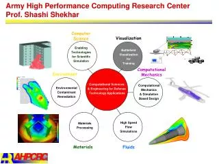
Research Goals Research Goals: • Find global climate patterns of interest to Earth Scientists A key interest is finding connections between the ocean and the land. • Global snapshots of values for a number of variables on land surfaces or water. • Monthly over a range of 10 to 50 years.
Patterns of Interest • Zone Formation • Find regions of the land or ocean which have similar behavior. • Teleconnections • Teleconnections are the simultaneous variation in climate and related processes over widely separated points on the Earth. • Associations • Find relations between climate events and land cover. • River Discharge • Relationship between water discharged from a river and precipitation, climate, and man.
Clustering for Zone Formation • Interested in relationships between regions, not “points.” • For ocean, clustering based on SST (Sea Surface Temperature) or SLP (Sea Level Pressure). • For land, clustering based on NPP or other variables, e.g., precipitation, temperature. • Typically we work with the points. • When “raw” NPP and SST are used, clustering can find seasonal patterns. • Anomalous regions have plant growth patterns which reversed from those typically observed in the hemisphere in which they reside, and are easy to spot.
K-Means Clustering of Raw NPP and Raw SST (Num clusters = 2) Land Cluster Cohesion: North = 0.78, South = 0.59 Ocean Cluster Cohesion: North = 0.77, South = 0.80
Preprocessing • Time series preprocessing issues • Need to remove seasonality • Earth scientists mostly interest in anomalies • Need to remove most of the autocorrelation • Statistical test are affected • Need to remove trends • Normally want to detect patterns and trends separately • Normally interested in similarity once differences in means and scale have been considered. • Pearson’s correlation coefficient has this property
Minneapolis Atlanta Sao Paolo Minneapolis 1.0000 0.7591 -0.7581 Minneapolis Atlanta 0.7591 1.0000 -0.5739 Sao Paolo -0.7581 -0.5739 1.0000 Sample NPP Time Series Correlations between time series
Minneapolis Atlanta Sao Paolo Minneapolis 1.0000 0.0492 0.0906 Minneapolis Atlanta 0.0492 1.0000 -0.0154 Sao Paolo 0.0906 -0.0154 1.0000 Seasonality Accounts for Much Correlation Normalized using monthly Z Score: Subtract off monthly mean and divide by monthly standard deviation Correlations between time series
Preprocessing: Removing Trends A slight linear trend added to two random time series increases their correlation dramatically, from 0.01 to 0.17.
© V. Kumar Discovery of Patterns in the Global Climate System using Data Mining 13 Ocean Climate Indices: Connecting the Ocean and the Land • An OCI is a time series of temperature or pressure • Based on Sea Surface Temperature (SST) or Sea Level Pressure (SLP) • OCIs are important because • They distill climate variability at a regional or global scale into a single time series. • They are well-accepted by Earth scientists. • They are related to well-known climate phenomena such as El Niño.
Ocean Climate Indices – ANOM 1+2 • ANOM 1+2 is associated with El Niño and La Niña. • Defined as the Sea Surface Temperature (SST) anomalies in a regions off the coast of Peru • El Nino is associated with • Droughts in Australia and Southern Africa • Heavy rainfall along the western coast of South America • Milder winters in the Midwest El Nino Events
Connection of ANOM 1+2 to Land Temp OCIs capture teleconnections, i.e., the simultaneous variation in climate and related processes over widely separated points on the Earth.
Ocean Climate Indices - NAO • The North Atlantic Oscillation (NAO) is associated with climate variation in Europe and North America. • Normalized pressure differences between Ponta Delgada, Azores and Stykkisholmur, Iceland. • Associated with warm and wet winters in Europe and in cold and dry winters in northern Canada and Greenland • The eastern US experiences mild and wet winter conditions. Iceland Azores
Influence of OCI on Land – Area Weighted Correlation • Correlation of an OCI with a land variable is a standard way to evaluate its “influence.” • Correlation does not imply causality. • Temperature and precipitation are the typical land variables. • If relatively many land points have a relatively high correlation, then an OCI is influential. • To evaluate whether clusters (or pairs) are potential OCIs we compute their area weighted correlation. • Weighted average of the correlation with land points, where weight is based on area. • May exclude points whose correlation is low and then calculate area weighted correlation.
Evaluation of Known OCIs via Area Weighted Correlation Area Weighted Correlation of Known OCIs to Land Temp Overlapping, threshold = 0
Discovery of Ocean Climate Indices • Use clustering to find areas of the oceans that have high density, I.e., relatively homogeneous behavior. • Cluster centroids are potential OCIs. • For SLP pairs of cluster centroids are potential OCIs. • Evaluate the “influence” of potential OCIs on land points. • Determine if the potential OCI matches a known OCI. • For potential OCIs that are not well-known, conduct further evaluation. • Are there land points that have higher correlation for the potential OCI than for known indices?
Evaluating Cluster Centroids as Potential OCIs • Evaluation will be based on area weighted correlation • Ignore clusters who area weighted correlation is low. • Three cases: • Clusters are highly similar to known OCIs (corr > 0.4) • May represent a known OCI • Clusters may be “better,” i.e., higher coverage • Clusters may cover different area, i.e., some points for which the new OCI is a better predictor • Clusters are moderately similar to known OCIs ( 0.25 < corr < 0.4 ) • Again, new OCIs may be better predictors for some points. • Clusters are not similar to known OCIs (corr < 0.25) • These clusters may represent as yet undiscovered Earth Science phenomena.
SST Clusters Highly Correlated to Known Indices Area Weighted Correlation of Cluster Centroids to Land Temp Overlapping, threshold = 0
SST Clusters that Correspond to El Nino Climate Indices 75 78 67 94 El Nino Regions Defined by Earth Scientists SNN clusters of SST that are highly correlated with El Nino indices, ~ 0.93 correlation.
SST Clusters Highly Correlated to Known Indices … Examples of some SST clusters that are highly correlated to known OCIs and have high area weighted correlation with land temperature. These indices have a significant correlation with El Nino indices.
SST Clusters Highly Correlated to Known Indices However, there are areas (yellow) where these clusters correlate better.
Mining Associations in Earth Science Data • First, transform Earth Science data into transactions. • Find patterns using association discovery algorithms. 1 FPAR-HI PET-HI PREC-HI SOLAR-HI TEMP-HI ==> NPP-HI (support count=145, confidence=100%) 2 FPAR-HI PET-HI PREC-HI TEMP-HI ==> NPP-HI (support count=933, confidence=99.3%) 3 FPAR-HI PET-HI PREC-HI ==> NPP-HI (support count=1655, confidence=98.8%) 4 FPAR-HI PET-HI PREC-HI SOLAR-HI ==> NPP-HI (support count=268, confidence=98.2%) … 75 FPAR-HI ==> NPP-HI (support count = 216924, confidence = 55.7%)
Example of Interesting Association Rules FPAR-Hi ==> NPP-Hi (sup=5.9%, conf=55.7%) Shrubland areas
Shrublands/ Land Cover Types
Example of Interesting Association Rules… Support Count Land Cover • Temp-Hi NPP-Hi tends to occur in the forest and cropland regions in the northern hemisphere (Forests (33.5%), Grassland(8.7%), Cropland (24.5%), Desert (0.4%) )
Gradient Analysis of SLP Data SLP in June, 1992
Trajectory Analysis of SST Data We choose a bounding box around the equatorial Pacific east of the dateline: longitude range: 80W -- 180W latitude range: 50N -- 15S Then, we calculated the locations of centroids of the top 20% SST cluster in the given region, and we plotted the trajectory albums for the centroid movements in one year.
Weather Data • Obtained from Barbara Broome. • Data • One day at 6 time periods • Grid is 51 x 51 units • 9.66 by 6.76 • Air temperature, pressure and two types of wind data