Download
1 / 40
400 likes | 480 Views
A Simple Model for the Solar Isorotation Countours. Steven A. Balbus Ecole Normale Supérieure Physics Department Paris, France. SOLAR DIFFERENTIAL ROTATION. One of the most beautiful astronomical results of the last half century was the precision determination

E N D
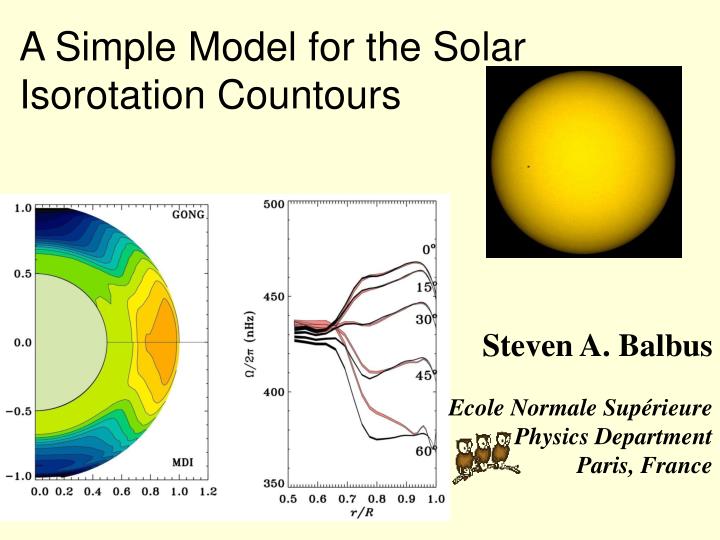
A Simple Model for the Solar Isorotation Countours Steven A. Balbus Ecole Normale Supérieure Physics Department Paris, France
SOLAR DIFFERENTIAL ROTATION • One of the most beautiful astronomical results of the last half century was the precision determination of the interior solar rotation. Splitting of p-mode frequencies allows an accurate determination of the angular velocity (r, ), using sophisticated inversion techniques applied to the excited mode spectrum.
THE FINDINGS: • The only place where there is significant differential rotation in the sun is in the convective zone (CZ). • This is thought to be the only place where there is a significant level of turbulence. (So much for enhanced viscosity models.) • The rotation is approximately constant on cones of constant at mid latitudes, cylindrical near the equator, spherical (apparently) near the poles.
Howe et al. 2000 “Tachocline” Surface shear
THE PROBLEM: • The CZ is very nearly adiabatic, P=P(), barotropic. • Convective motions, except near the surface, are small… typically 30 m s-1. • A barotropic fluid in hydrostatic equilibrium must rotate on cylinders, ( R ). (Taylor columns.) The solar rotation profile is decidedly not constant on cylinders. • But large scale numerical simulations generally do produce cylindrical contours.
Brun & Toomre 2002 ASH Code Miesch, 2007
THE ORTHODOX VIEW • Despite the simple regularity of the rotation pattern, the flow is an extremely complex interplay between convective turbulence and rotation. Some handles exist, however. • Departures from barotropic structure because Coriolis forces affect convection. • Convection along the axis of rotation is more efficient than convection in planes of constant Z. Hot poles, cool equator. • Thermal wind equation: R Ω2/z = e· (P )/ 2
THERMAL WIND EQUATION R Ω2/z = e· (P )/ 2 ; (R, , z) or (r, , ) R 2Ω2/z = (/r) (P/r) - (/r) (P/r) Let S = k/(-1) ln P- , CP = k/(-1) , R CP Ω2/z = (P/r) (S/r) - (P/r) (S/r) For SCZ: RCP Ω2/z = g (S/r) , g= - (P/r). Shows relationship between large scale latitudinal entropy gradients due to Coriolis, and departures from cylindrical “isotachs.” Trend: moving polewards, Ω dec., S inc.
GETTING THE LAY OF THE LAND N2 = | g/ (ln P- ) /r | ≈ 3.8 X 10⁻¹³ s-2, by requiring the solar luminosity to be carried by convection (Schwarzschild 1958). But gradient of S is estimated by different TWE physics… g/ (ln P- ) /r = RΩ2/z ≈ 2 X 10-12 s-2, The gradient of S exceeds the r gradient by factor of ~ 5…if thermal wind balance is valid.
S, Ω COUNTER ALIGNED ? Clearly, e Ω also much exceeds er Ω . er Ω
S, Ω COUNTER ALIGNED ? Clearly, e Ω also much exceeds er Ω . What if Ω and S are more closely related than just a trend? What if S=S(Ω2) ? S er Ω
Thermal Wind Equation with S=S(Ω2): where S’ is dS/dΩ2. Solution is Ω2 is constant along the characteristic Since Ω is constant along this characteristic, so is S’. To solve, set y = sin . Find: , a first order linear equation.
The basic result is clear: R small, r=const. r >> B/2A, R=const. With g=GM/r2, the solution is: where A is an integration constant, and B is B/r3 ~ order unity or less.
With g=GM/r2, the solution is: where A is an integration constant, and B is B/r3 ~ order unity or less. For solving for Ω, assume a fit at r=r, Ω(cos2o), where o is at r=r, the starting point of the characteristic
“Batman contour” is typical. Spheres at small R, cylinders at larger R, sharp upturn in between.
0.2 0.1 0.4 0.3
0.5 0.6 0.7 0.8
Thermal Wind Equation for S=S(L2): Solution is angular momentum is const. along characteristic Solution is similar to angular velocity characteristics. Find:
0.1 0.2 0.4 0.3
This is often the way it is in physics---our mistake is not that we take our theories too seriously, but that we do not take them seriously enough. ---Steven Weinberg, in The First Three Minutes
HOW IS IT THAT S AND Ω CARE ABOUT EACH OTHER SO MUCH? To answer this, we need to understand something about the stability of rotating, stratified, magnetized plasmas. We need to take rotation, stratification and magnetism seriously.
THE PUNCHLINE: Counter alignment of the entropy and angular velocity gradients is a rigorous condition for marginal stability in a rotating, convective, magnetized gas.
THE PUNCHLINE: The solar rotation profile can be understood as a consequence of maintaining a state of marginal (in)stability to the most rapidly growing axi- and nonaxisymmetric dynamical modes.
THE PUNCHLINE: A magnetic field is essential to this picture.
Fundamental linear response of a magnetized medium: (Boussinesq; degenerate Alfvén & slow modes.) Addition of rotation introduces two new terms, one of which is “epicyclic,” 2=d2/dlnR +42, the other of which is “tethering,” and gives rise to the MRI.
Schematic MRI 2 angular momentum 1 To rotation center
2 1 Schematic MRI angular momentum To rotation center
Compact form of equation: General wave numbers: Allow Ω(R, z):
Allow S(R,z) as well: Most general, barotropic, axisymmetric response. Stability from limit:
More clear written in terms of displacement vector, n Then, Marginal modes exist when rotation and entropy surfaces coincide. Explicitly (Papaloizou & Szuszkiewicz 1992, Balbus 1995): + + - - N2 + dΩ2/dln R >0 also required, but amply satisfied.
Did we miss something? What happened to good old-fashioned convection? Marginalization of BV oscillations picked out by nonaxisymmetric modes. Without a magnetic field, these purely hydrodynamic modes dominate the question of stability. With even a weak magnetic field, the axisymmetric modes become major players.
Z S S S stable stable unstable R Ω Ω Ω
(k•vA)2 unstable zone R/z (kvA)2 versus R/z under conditions of marginal instability
Global Simulations of the MRI, Hawley 2000 Equatorial Plane Meridional Plane
SUMMARY & SYNTHESIS • A dominant balance of the vorticity equation • corresponding to the thermal wind equation seems • to hold in much of the SCZ. • 2. Implies S/ >> S/ ln r , just as seen in Ω contours. • TWE equation may be solved exactly with S=S(Ω ). Produces isorotation contours in broad agreement with helioseismology. • As it happens, S=S(Ω ) corresponds precisely to marginal stability of axisymmetric, baroclinic, magnetized modes in rotating gas. Coincidence?
SUMMARY & SYNTHESIS • 5. Nonaxisymmetric modes couple to N2, but insensitive to • magnetic couplings. Axisymmetric modes couple strongly to • rotation, very sensitive to magnetic field. Hydro stability criteria • very different, not near criticality. • The gross dynamical (“Batman isotachs”) and thermal (adiabatic) features of the SCZ are a consequence of marginalizing the dominant magnetobaroclinic linear unstable modes of the system.
SUMMARY & SYNTHESIS • Need to resolve (kvA)2 = ∂Ω2 /∂ ln R wavelengths , nominally difficult, not impossible. Can surely fudge parameters to bring into computational domain. Calibration with linear dispersion relation is essential. • Ideas are generic, simple. For the future, hope is that they will prove to be useful for problems they were not designed to solve directly, e.g. latitude dependence of dynamo cycle N2(r, ). (M. McIntyre).