Download
1 / 22
220 likes | 277 Views
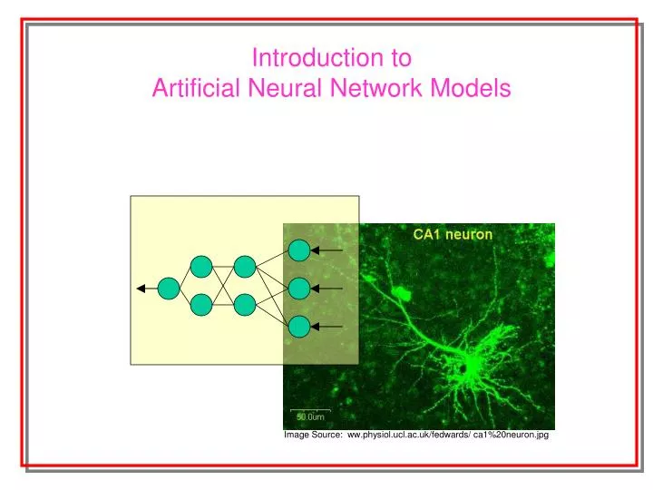
Image Source: ww.physiol.ucl.ac.uk/fedwards/ ca1%20neuron.jpg. Introduction to Artificial Neural Network Models. Definition. Neural Network A broad class of models that mimic functioning inside the human brain. There are various classes of NN models.

E N D
Image Source: ww.physiol.ucl.ac.uk/fedwards/ ca1%20neuron.jpg Introduction to Artificial Neural Network Models
Definition Neural Network A broad class of models that mimic functioning inside the human brain • There are various classes of NN models. • They are different from each other depending on • Problem types Prediction, Classification , Clustering • Structure of the model • Model building algorithm For this discussion we are going to focus on Feed-forward Back-propagation Neural Network (used for Prediction and Classification problems)
Dendrites Cell Body Axon Synapse A bit of biology . . . Most important functional unit in human brain – a class of cells called – NEURON Hippocampal Neurons Source: heart.cbl.utoronto.ca/ ~berj/projects.html Schematic • Dendrites – Receive information • Cell Body – Process information • Axon – Carries processed information to other neurons • Synapse – Junction between Axon end and Dendrites of other Neurons
f An Artificial Neuron Dendrites Cell Body Axon X1 Direction of flow of Information w1 w2 X2 V = f(I) I . . . I = w1X1 +w2X2 +w3X3 +… + wpXp wp Xp • Receives Inputs X1 X2 …Xp from other neurons or environment • Inputs fed-in through connections with ‘weights’ • Total Input = Weighted sum of inputs from all sources • Transfer function (Activation function) converts the input to output • Output goes to other neurons or environment
1 1 0.5 0 -1 Transfer Functions There are various choices for Transfer / Activation functions 1 0 Logistic f(x) = ex / (1 + ex) Threshold 0 if x< 0 f(x) = 1 if x >= 1 Tanh f(x) = (ex – e-x) / (ex + e-x)
X1 X2 X3 X4 Direction of information flow y1 y2 ANN – Feed-forward Network A collection of neurons form a ‘Layer’ Input Layer - Each neuron gets ONLY one input, directly from outside Hidden Layer - Connects Input and Output layers Output Layer - Output of each neuron directly goes to outside
ANN – Feed-forward Network Number of hidden layers can be None One More
X1 X2 X3 X4 y1 y2 ANN – Feed-forward Network Couple of things to note • Within a layer neurons are NOT connected to each other. • Neuron in one layer is connected to neurons ONLY in the NEXT layer. (Feed-forward) • Jumping of layer is NOT allowed
One particular ANN model What do we mean by ‘ A particular Model ‘ ? Input: X1 X2 X3 Output: Y Model: Y = f(X1 X2 X3) For an ANN : Algebraic form of f(.) is too complicated to write down. • However it is characterized by • # Input Neurons • # Hidden Layers • # Neurons in each Hidden Layer • # Output Neurons • WEIGHTS for all the connections ‘ Fitting ‘ an ANN model = Specifying values for all those parameters
X2 X3 X1 -0.2 0.6 -0.1 0.1 0.7 0.5 0.1 -0.2 Y Decided by the structure of the problem # Input Nrns = # of X’s # Output Nrns = # of Y’s Free parameters One particular Model – an Example Model: Y = f(X1 X2 X3) Input: X1 X2 X3 Output: Y Parameters Example # Input Neurons 3 # Hidden Layers 1 # Hidden Layer Size 3 # Output Neurons 3 Weights Specified
X1 =1 X2=-1 X3 =2 0.2 = 0.5 * 1 –0.1*(-1) –0.2 * 2 f(x) = ex / (1 + ex) f(0.2) = e0.2 / (1 + e0.2) = 0.55 0.2 0.9 Predicted Y = 0.478 f (0.9) = 0.71 f (0.2) = 0.55 0.55 0.71 -0.087 f (-0.087) = 0.478 0.478 Prediction using a particular ANN Model Input: X1 X2 X3 Output: Y Model: Y = f(X1 X2 X3) -0.2 0.6 -0.1 0.1 0.7 0.5 0.1 -0.2 Suppose Actual Y = 2 Then Prediction Error = (2-0.478) =1.522
# Hidden Layer = ??? Try 1 # Neurons in Hidden Layer = ???Try 2 No fixed strategy. By trial and error Building ANN Model How to build the Model ? Input: X1 X2 X3 Output: Y Model: Y = f(X1 X2 X3) # Input Neurons = # Inputs = 3 # Output Neurons = # Outputs = 1 Architecture is now defined … How to get the weights ??? Given the Architecture There are 8 weights to decide. W = (W1, W2, …, W8) Training Data: (Yi , X1i, X2i, …, Xpi ) i= 1,2,…,n Given a particular choice of W, we will get predicted Y’s ( V1,V2,…,Vn) They are function of W. Choose W such that over all prediction error E is minimized E = (Yi – Vi) 2
Start with a random set of weights. • Feed forward the first observation through the net X1 Network V1 ; Error = (Y1 – V1) • Adjust the weights so that this error is reduced ( network fits the first observation well ) • Feed forward the second observation. Adjust weights to fit the second observation well • Keep repeating till you reach the last observation • This finishes one CYCLE through the data • Perform many such training cycles till the overall prediction error E is small. Back Propagation Feed forward Training the Model How to train the Model ? E = (Yi – Vi) 2
Back Propagation Bit more detail on Back Propagation Each weight ‘Shares the Blame’ for prediction error with other weights. Back Propagation algorithm decides how to distribute the blame among all weights and adjust the weights accordingly. Small portion of blame leads to small adjustment. Large portion of the blame leads to large adjustment. E = (Yi – Vi) 2
Weight adjustment during Back Propagation Weight adjustment formula in Back Propagation Vi – the prediction for ith observation – is a function of the network weights vector W= ( W1, W2,….) Hence, E, the total prediction error is also a function of W E( W) = [ Yi – Vi( W ) ] 2 Gradient Descent Method : For every individual weight Wi, updation formula looks like Wnew = Wold + * ( E / W) |Wold = Learning Parameter (between 0 and 1) Another slight variation is also used sometimes W(t+1) = W(t) + * ( E / W) |W(t) + * (W(t) - W(t-1) ) = Momentum (between 0 and 1)
w1 w2 Geometric interpretation of the Weight adjustment Consider a very simple network with 2 inputs and 1 output. No hidden layer. There are only two weights whose values needs to be specified. E( w1, w2) = [ Yi – Vi(w1, w2 ) ] 2 • A pair ( w1, w2 ) is a point on 2-D plane. • For any such point we can get a value of E. • Plot E vs ( w1, w2 ) - a 3-D surface - ‘Error Surface’ • Aim is to identify that pair for which E is minimum • That means – identify the pair for which the height of the error surface is minimum. • Gradient Descent Algorithm • Start with a random point ( w1, w2 ) • Move to a ‘better’ point ( w’1, w’2 ) where the height of error surface is lower. • Keep moving till you reach ( w*1, w*2 ), where the error is minimum.
Error Surface Local Minima Global Minima w* w0 Weight Space Crawling the Error Surface
Do till Convergence criterion is not met For I = 1 to # Training Data points Next I End Do Training Algorithm Decide the Network architecture (# Hidden layers, #Neurons in each Hidden Layer) Decide the Learning parameter and Momentum Initialize the Network with random weights Feed forward the I-th observation thru the Net Compute the prediction error on I-th observation Back propagate the error and adjust weights E = (Yi – Vi) 2 Check for Convergence
Convergence Criterion When to stop training the Network ? Ideally – when we reach the global minima of the error surface How do we know we have reached there ? We don’t … • Suggestion: • Stop if the decrease in total prediction error (since last cycle) is small. • Stop if the overall changes in the weights (since last cycle) are small. Drawback: Error keeps on decreasing. We get a very good fit to training data. BUT … The network thus obtained have poor generalizing power on unseen data The phenomenon is also known as - Over fitting of the Training data The network is said to Memorize the training data. - so that when an X in training set is given, the network faithfully produces the corresponding Y. -However for X’s which the network didn’t see before, it predicts poorly.
Validation Error Training Cycle Convergence Criterion Modified Suggestion: Partition the training data into Training set and Validation set Use Training set - build the model Validation set - test the performance of the model on unseen data Typically as we have more and more training cycles Error on Training set keeps on decreasing. Error on Validation set keeps first decreases and then increases. Stop training when the error on Validation set starts increasing
Choice of Training Parameters Learning Parameter and Momentum - needs to be supplied by user from outside. Should be between 0 and 1 What should be the optimal values of these training parameters ? - No clear consensus on any fixed strategy. - However, effects of wrongly specifying them are well studied. Learning Parameter Too big – Large leaps in weight space – risk of missing global minima. Too small – - Takes long time to converge to global minima - Once stuck in local minima, difficult to get out of it. Suggestion Trial and Error – Try various choices of Learning Parameter and Momentum See which choice leads to minimum prediction error
Wrap Up • Artificial Neural network (ANN) – A class of models inspired by biological Neurons • Used for various modeling problems – Prediction, Classification, Clustering, .. • One particular subclass of ANN’s – Feed forward Back propagation networks • Organized in layers – Input, hidden, Output • Each layer is a collection of a number of artificial Neurons • Neurons in one layer in connected to neurons in next layer • Connections have weights • Fitting an ANN model is to find the values of these weights. • Given a training data set – weights are found by Feed forward Back propagation algorithm, which is a form of Gradient Descent Method – a popular technique for function minimization. • Network architecture as well as the training parameters are decided upon by trial and error. Try various choices and pick the one that gives lowest prediction error.