Download
1 / 44
460 likes | 629 Views
Introduction to Learning Classifier Systems. Dr. J. Bacardit, Dr. N. Krasnogor G53BIO - Bioinformatics. Outline. Introduction Machine Learning & Classification Paradigms of LCS Knowledge representations Real-world examples Recent trends Summary. Introduction.

E N D
Introduction to Learning Classifier Systems Dr. J. Bacardit, Dr. N. Krasnogor G53BIO - Bioinformatics
Outline • Introduction • Machine Learning & Classification • Paradigms of LCS • Knowledge representations • Real-world examples • Recent trends • Summary
Introduction • Learning Classifier Systems (LCS) are one of the major families of techniques that apply evolutionary computation to machine learning tasks • Machine learning: How to construct programs that automatically learn from experience [Mitchell, 1997] • LCS are almost as ancient as GAs, Holland made one of the first proposals
Introduction • Paradigms of LCS • The Pittsburgh approach [Smith, 80] • The Michigan approach [Holland & Reitman, 78] • The Iterative Rule Learning approach [Venturini, 93] • Knowledge representations • All the initial approaches were rule-based • In recent years several knowledge representations have been used in the LCS field: decision trees, synthetic prototypes, etc.
Machine Learning and classification • A more formal definition of machine learning and some examples [Mitchell, 1997] • A computer program is said to learn from experience E with respect to some class of tasks T and performance measure P, if its performance at tasks in T, as measured by P, improves with experience E • How does this definition translate to real life?
Machine Learning and classification • A checkers learning problem • Task T: playing checkers • Performance measure P: percent of games won against opponents • Training experience E: playing practice games against itself
Machine Learning and classification • A handwriting recognition learning problem • Task T: recognizing and classifying handwritten words withing images • Performance measure P: percent of words correctly identified • Training experience E: a database of handwritten words with given classifications
Machine Learning and classification • A robot driving learning problem • Task T: driving on public four-lane highways using vision sensors • Performance measure P: average distance traveled before an error (as judged by human overseer) • Training experience E: a sequence of images and steering commands recorded while observing a human driver
New Instance Training Set Learning Algorithm Inference Engine Class Machine Learning and classification • Classification task: Learning how to label correctly new instances from a domain based on a set of previously labeled instances
Machine Learning and classification • Instance: individual, independent example of the domain that has to be learned • Instances have regular structure: • Fixed number of attributes: features that characterize an instance • A class: a label belonging to a finite and discrete domain • Attributes can be of diverse type • Nominal: discrete and finite variable • Integer • Continuous
Machine Learning and classification • Instance • Goal of classification is to learn how to predict the class of an instance from its attributes An A1 A2 Class A B . . E 2 classes n classes [n..m]
Machine Learning and classification 1 Instance: (X,Y||Colour) 1: If (X<0.25 and Y>0.75) or (X>0.75 and Y<0.25) then Y 2: If (X>0.75 and Y>0.75) then 3: If (X<0.25 and Y<0.25) then 4: If (X [0,25,0,50] and Y [0.25,0.50]) then 4’: Everything else then 0 1 X
Paradigms of LCS • Paradigms of LCS • The Pittsburgh approach [Smith, 80] • The Michigan approach [Holland & Reitman, 78] • The Iterative Rule Learning approach [Venturini, 93]
Paradigms of LCS • The Pittsburgh approach • This approach is the closest one to the standard concept of GA • Each individual is a complete solution to the classification problem • Traditionally this means that each individual is a variable-length set of rules • GABIL [De Jong & Spears, 93] is a well-known representative of this approach
Paradigms of LCS • Pittsburgh approach • More than one rule could be used to classify a given instance • Match process: deciding which rule is used in these cases • An usual approach is that individuals are interpreted as a decision list [Rivest, 87]: an ordered rule set Instance 1 matches rules 2, 3 and 7 Rule 2 will be used Instance 2 matches rules 1 and 8 Rule 1 will be used Instance 3 matches rule 8 Rule 8 will be used Instance 4 matches no rules Instance 4 will not be classified 1 2 3 4 5 6 7 8
Paradigms of LCS • Pittsburgh approach • Crossover operator • Mutation operator: classic GA mutation of bit inversion Offspring Parents
Paradigms of LCS • Pittsburgh approach • Evaluation process of an individual: • NumExamples=0 • CorrectExamples=0 • For each example in training set • NumExamples++ • Determine first rule that matches training example • If class of rule is the same as class of instance • CorrectExamples++ • Fitness=(CorrectExamples/NumExamples)2
Paradigms of LCS • In the other two approaches each individual is a rule • What happens usually in the evolutionary process of a GA? • All individuals converge towards a single solution • Our solution is a set of rules. Therefore we need some mechanism to guarantee that we generate all of them. • Each approach uses a different method for that
Paradigms of LCS • The Michigan approach • Each individual (classifier) is a single rule • The whole population cooperates to solve the classification problem • A reinforcement learning system is used to identify the good rules • A GA is used to explore the search space for more rules • XCS [Wilson, 95] is the most well-known Michigan LCS
Paradigms of LCS • The Michigan approach • What is Reinforcement Learning? • “a way of programming agents by reward and punishment without needing to specify how the task is to be achieved” [Kaelbling, Littman, & Moore, 96] • Rules will be evaluated example by example, receiving a positive/negative reward • Rule fitness will be update incrementally with this reward • After enough trials, good rules should have high fitness
Paradigms of LCS • Working cycle
Paradigms of LCS • The Iterative Rule Learning approach • Each individual is a single rule • Individuals compete as in a standard GA A single GA run generates one rule • The GA is run iteratively to learn all rules that solve the problem • Instances already covered by previous rules are removed from the training set of the next iteration
Paradigms of LCS • The Iterative Rule Learning approach • Also known as separate-and-conquer Partial Training set Remove covered examples No All examples covered? Initial Training set Add rule to rule set Generate one rule Yes Rule set Learning finished
Paradigms of LCS • The Iterative Rule Learning approach • HIDER System [Aguilar, Riquelme & Toro, 03] • Input: Examples • RuleSet = Ø • While |Examples| > 0 • Rule = Run GA with Examples • RuleSet = RuleSet U Rule • Examples = Examples \ Covered(Rule) • EndWhile • Output: RuleSet • Fitness uses accuracy + generality measure • Generality: rule covering as much examples as possible
Knowledge representations • Knowledge representations • For nominal attributes • Ternary representation • GABIL representation • For real-valued attributes • Decision tree • Synthetic prototypes • Others
Knowledge representations • Representation of XCS for binary problems: ternary representation • Ternary alphabet {0,1,#} • If A1=0 and A2=1 and A3 is irrelevant class 0 • For non-binary nominal attributes: • {0,1, 2, …, n,#} • Crossover and mutation act as in a classic GA 01#|0
Knowledge representations • Representation of GABIL for nominal attributes • Predicate Class • Predicate: Conjunctive Normal Form (CNF) (A1=V11.. A1=V1n) ..... (An=Vn2.. An=Vnm) • Ai : ith attribute • Vij : jth value of the ith attribute • The rules can be mapped into a binary string 1100|0010|1001|1 • Usual crossover and mutation
Knowledge representations • Representation of GABIL for nominal attributes • 2 Variables: • Sky = {clear, partially cloudy, dark clouds} • Pressure = {Low, Medium, High} • 2 Classes: {no rain, rain} • Rule: If [sky is (partially cloudy or has dark clouds)] and [pressure is low] then predict rain • Genotype: “011|100|1”
Knowledge representations • Representation of XCS for real-valued attributes: real-valued interval • XCSR [Wilson, 99] • Interval is codified with two variables: center & spread: [center, spread] [center-spread,center+spread] • Rule for the colours example: • [0.125,0.125]|[0.125,0.125]| • Usual crossover • Mutation adds or substracts a small quantity from the genes
Knowledge representations • Representation of XCS for real-valued attributes: real-valued interval • UBR [ Stone & Bull, 03] • Interval is codified with two variables: lower & upper bound: [lower, upper] • The variable with lowest value is the lower bound, the variable with higher value is the upper bound • [0,0.25]|[0.25,0]|
Knowledge representations • Pittsburgh representations for real-valued attributes: • Rule-based: Adaptive Discretization Intervals (ADI) representation [Bacardit, 04] • Intervals in ADI are build using as possible bounds the cut-points proposed by a discretization algorithm • Search bias promotes maximally general intervals • Several discretization algorithms are used at the same time in order to choose correctly the appropiate method for each domain
Knowledge representations • Pittsburgh representations for real-valued attributes: • Decision trees [Llorà, 02] • Nodes in the trees can use orthogonal or oblique criteria
Knowledge representations • Pittsburgh representations for real-valued attributes: • Orthogonal decision tree 1 X X>0.5 X<0.5 Y Y Y<0.5 Y>0.5 0 1 X
Knowledge representations • Pittsburgh representations for real-valued attributes • Synthetic prototypes [Llorà, 02] • Each individual is a set of synthetic instances • These instances are used as the core of a nearest-neighbor classifier ?
Pittsburgh representations for real-valued attributes • Synthetic prototypes 1 • (-0.125,0,yellow) • (0.125,0,red) • (0,-0.125,blue) • (0,0.125,green) Y -1 0 1
Real-world applications • Generating control rules for a fighter aircraft [Smith et. al., 00] • Using Michigan LCS • Learning aircraft maneuvers • Input information: • Airspeed, altitude, aircraft angle, … • Actions (classes): • Rudder angle and speed
Real-world applications • Predicting the mill temperature (range of temperatures) in a aluminium plate mill [Browne & Bacardit, 04] • The Pittsburgh approach was used • A press is used to level raw aluminium into a thin sheet that can be coiled • The aluminium temperature should be within some operational limits • Temperature is predicted from around 60 input sensors
Real-world applications • Medical domains: Generation of epidemiologic hypothesis [Holmes, 96] • Predicting if a pacient has a disease based on their degree of exposure to certain factors • In this domain the difference between false positives and false negatives is important
Recent trends • Develop a theoretical framework of the behavior of each kind of LCS • These models are intended to allow the user to adjust the LCS in a principled way to guarantee success • Convert LCS into an engineering tool
Recent trends • New kinds of knowledge representations, specially non-linear ones • Making sure that the representation has enough expressive power to model successfully the domain
Recent trends • Development of exploration mechanism that can go beyond the classic crossover and mutation operators • It is known that these classic exploration mechanisms have limitations, specially in identifying the structure of the problem • If the algorithm learns this structure, it can explore more efficiently and find better solutions
Summary • This talk was a brief overview of the Learning Classifier Systems area: EC techniques applied to Machine Learning • Description of the three main paradigms • Pittsburgh • Michigan • Iterative rule learning
Summary • Description of several knowledge representations • Rule based • Nominal attributes • Continuous attributes • Decision trees • Synthetic prototypes
Summary • Applications to real-world domains • Medical • Industrial • Military • Recent trends • Explore better • Model the problem better • Understand better