Download

1 / 8
80 likes | 86 Views
Guidelines to problems chapter 9. Nutan S. Mishra Department of mathematics and Statistics University of South Alabama. Important points to remember. X is a random variable with parameters µ and σ .

E N D
Guidelines to problems chapter 9 Nutan S. Mishra Department of mathematics and Statistics University of South Alabama
Important points to remember • X is a random variable with parameters µ and σ. • In fact X represent the whole population (of some laaarge size) whose average is µ with standard deviation σ • µ and σ are parameters of the population which is represented by X • For a given population values of parameters are always fixed • For a given population values of parameters are often unknown. • So we collect a sample of size n from this population • In fact we could collect hundreds of such samples from the population. • And for each such sample we could compute the sample mean and sample standard deviation s • The value of sample mean is different for different samples • Thus we have a large group of sample means. • All the sample means form a new population represented by • This new population of sample means represented by has mean and standard deviation • The values of the population parameters of the new random variable are given by = µ and = σ/√n
Exercise 9.9 • H0: µ = 20 hours vs H1: µ ≠ 20 hours, this is a two tailed test. • H0: µ = 10 hours vs H1: µ ≠ 10 hours, this a two tailed test. • H0: µ = 3 years vs H1: µ ≠ 3 years, this is a two tailed test • H0: µ = $1000 vs H1: µ < $1000, this is a left tailed test. • H0: µ = 12 minutes vs H1: µ > 12 minutes, this is a right tailed test.
Exercise 9.17 Size of population = 8.1 million X= duration of unemployment for the people of 16 and over ( note that µ and σ are unknown) Size of sample n = 400 sample mean = 16.9 weeks sample s.d. = s=4.2 weeks (note that sample size is large) To test H0: µ = 16.3 weeks Vs H1: µ > 16.3 weeks Given that size of rejection region is α= .02 Note that this is a right tailed test. Since the sample size is large, we choose the z-distribution (standard normal) Thus the test statistic would be z = Since σ is unknown, we replace it by the sample standard deviation s = 4.2 weeks Thus z = = 2.86 and p-value = .0021 Since p-value < α , we make decision to reject H0 at 2% LOS And conclude that at 2% LOS the sample data does not support the H0 hence current duration of unemployment is greater than 16.3 weeks
Exercise 9.42 Population : households in United states. X= amount spent on gifts etc by a house hold during holiday season. In the year 2001 µ = $940 To test if the average amount spent this year is different from 2001. That is to test H0: µ = $940 vs H1 : µ ≠ $940 To test this hypothesis, they recently collected a sample Size of sample n = 324 households. = $1005, s = $330 Size of rejection region α = .01 Note that sample size is large , thus we choose z- distribution also test is two tailed. Thus our test statistic is z = Thus z= = 3.55 p-value = 2*.0002 = .0004 Since p-value << α , we make a decision to reject H0 And conclude that since sample data is not supporting null, the average expenditure by all households in United states on gifts etc, has increased since 2001.
Exercise 9.67 Population: female college basketball players. X= height of a player Assumption: x has normal distribution According to coach : µ = 69.5 inches To test this claim, a sample is collected with n = 25 players = 70.25 inches sample standard deviation = 2.1 inches α= .01 H0: µ = 69.5 inches vs H1: µ ≠ 69.5 inches Note that • Population is normal • Population standard deviation σ is unknown • Sample size is small Under these three conditions the test statistic follows t-distribution with n-1 d.f. Thus the test statistics t = follows t-distribution with 24 d.f. t = = 1.79 This is a two tailed test , p-value = 2* .05 (approximately) = .10 approximately Using flash apps on TI-89 exact p-value = .086 Since p-value >> α , we make a decision not to reject H0 at 1%LOS Conclude that at !% LOS sample data supports null that is average height is 69.5
Exercise 9.99 Population: Affluent Americans (annual income ≥ $75,000) X= # of households having serious problems in paying unexpected bill 0f $5000 According to “Money” Survey in 2002 , population proportion of such households p = .32 Question: has this proportion gone up since 2002? H0: p = .32 vs H1 : p > .32 In a recent survey they collected a sample of n = 1100 households with X = 396 that is sample proportion = 396/1100 = .36 To test the pair of hypotheses we have to choose a distribution first. Before choosing a distribution we need to decide if the sample size is large enough Here np = 1100* 0.32 = 352 and nq = 1100* (1-.32) = 748 Since both np and nq are larger than 5 the sample is large. Since the sample size is large, we choose z- (standard Normal) distribution and the test statistic is z = = = 2.84 hence p-value = .0023 Since p-value << α (which is .025) we make a decision to reject H0 And conclude that at 2.5% LOS data does not support the H0 hence the proportion of such people has gone up since 2002
Exercise 9.99 (b) Type I error = decide that population proportion has gone up when in fact it has not. P(type I error ) = α = .025