Download
1 / 17
170 likes | 265 Views
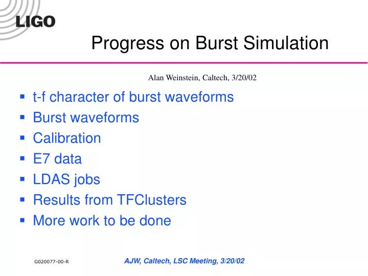
Progress on Burst Simulation. Alan Weinstein, Caltech, 3/20/02. t-f character of burst waveforms Burst waveforms Calibration E7 data LDAS jobs Results from TFClusters More work to be done. t-f character of burst waveforms (relevant for astrophysics-based analysis).

E N D
Progress on Burst Simulation Alan Weinstein, Caltech, 3/20/02 • t-f character of burst waveforms • Burst waveforms • Calibration • E7 data • LDAS jobs • Results from TFClusters • More work to be done AJW, Caltech, LSC Meeting, 3/20/02
t-f character of burst waveforms (relevant for astrophysics-based analysis) • Generic statements about the sensitivity of our searches to poorly-modeled sources can straightforwardly be made from the t-f “morphology”… • longish-duration, small bandwidth (chirps, ringdowns) • short duration, large bandwidth (merger) • In-between (ZM waveforms) • Of course, depends on t-f resolution, which must be optimized AJW, Caltech, LSC Meeting, 3/20/02
Waveforms buried in E2 noise, including calibration/TF chirp ZM supernova Hermite-gaussian ringdown AJW, Caltech, LSC Meeting, 3/20/02
Z-M waveforms (un-normalized) AJW, Caltech, LSC Meeting, 3/20/02
Burst waveforms • Start with simple, easy to interpret waveforms: damped sinusoids have well-defined central frequency and bandwidth: • h(t) = hpeak exp(-t/t) sin(2pfcent t), BW = 1/t • Choose narrow bandwidth for now, t = 0.1 sec, BW = 10 Hz • Scan over range of fcent, hpeak • Consider other bandwidths, other waveforms, later. • Since we’re analyzing lots of data (~512 secs) per job, inject multiple waveforms in one job, so that we don’t have to run so many jobs… • BUT, if these waveforms are BIG, and if the DSO calculates average power using the data itself, many injected waveforms could throw it off… • For now, this is just a convenience… AJW, Caltech, LSC Meeting, 3/20/02
Burst scan The first 2 waveforms, with fcent = 50 and 100 Hz; t=0.1 sec 32 waveforms, each 2 sec long, Scanning from 50 to 1600 Hz in 50 Hz steps. ASD of this 64-sec stretch of simulated data. Spectrogram to illustrate the frequency scan AJW, Caltech, LSC Meeting, 3/20/02
E7 data • Want to run at MIT • GUILD reports that at MIT, we have • 693960000 693967184 H R gwf /export/E7/LHO/frames • 693960000 693967184 L R gwf /export/E7/LLO/frames • These are 2 hrs of data from 1/1/02, when all 3 IFOs are in lock. • This is not playground data. We need playground data at MIT. • In the meantime, I choose a 361-sec stretch, since TFCLUSTERS apparently likes to run on that much data (I need to learn how to change that, if possible): 693961586-693961946, H2:LSC-AS_Q . (This stretch has lots of noise bursts). 8192 Hz 361 sec AJW, Caltech, LSC Meeting, 3/20/02
Injecting bursts • The burst signals are absolutely normalized by hpeak. Need to put it into same units as H2:LSC-AS_Q (volts) by using response function, obtained from calibration. • The burst signals are passed through a linear filter implementing the E7 H2 calibration transfer function, then saved to a frame file and ftp’ed to • http://www-ldas.mit.edu/ldas_outgoing/jobs/ldasmdc_data/burst-stochastic/burstscan_e7h2.F • Add signals to the data in LDAS DatacondAPI; can scale magnitude of signals as desired, at run-time. -framequery { { R H {} $times Adc($channel) } { F H /ldas_outgoing/jobs/ldasmdc_data/burst-stochastic/burstscan_e7h2.F {} Adc(0) } } -aliases { x = _ch0; s = _ch1; } -algorithms { zx = slice(x,0,5914624,1); zy = slice(s,0,5914624,1); zm = mul(zy,1.e0); zs = add(zx,zm); zz = tseries(zs, 16384.0, $stime, 0); pz = psd(zz,16384); intermediate(,pzs.ilwd,pz,psd of ch0); z = resample(zz,1,8); m = mean(z); y = sub(z,m); q = linfilt(b,y); r = slice(q,2047,737280,1); } AJW, Caltech, LSC Meeting, 3/20/02
E7 calibration http://blue.ligo-wa.caltech.edu/engrun/Calib_Home/ No calibration info from LLO has been posted here yet. AJW, Caltech, LSC Meeting, 3/20/02
Add bursts to data Time series Calibrated strain noise spectrum Noise spectrum Ratio of noise spectra, With/without injected signal AJW, Caltech, LSC Meeting, 3/20/02
BIG Bursts added to E7 data(as a check) Noise ASD for 361 secs of H2:LSC-AS_Q (red), And with BIG bursts added during secs 201-264 (blue). Bursts are added, and PSDs obtained, using LDAS/DataCond (thanks to Philip Charlton for his help). Strain sensitivity from 361 secs of H2:LSC-AS_Q (red), And with BIG bursts added (blue). Note that red curve is in good qualitative agreement with spectrum in Calib page, and bursts scan frequencies from 50-1600 Hz in 50 Hz steps, bandwidth = 10 Hz, and all with same peak strain. AJW, Caltech, LSC Meeting, 3/20/02
DSO search • Run with TFCLUSTERS, 361 seconds at a time. • Run on 361 sec data segment from H2, no injected signals: • 357 triggers into mit_test sngl_bursts table. • Inject 32 bursts with hpeak = 110-16 , scanning fcent from 50 to 1600 Hz in 50 Hz steps, signals spaced 2 secs apart, starting at sec 200. • 471 triggers into mit_test sngl_bursts table. Most big SNR triggers are unchanged after injection of simulated bursts. Many of the first 16 bursts stand out over the fakes. AJW, Caltech, LSC Meeting, 3/20/02
Efficiencies:Presenting the results Find loudest trigger within 1 sec of injected burst. Plot SNR vs frequency of injected burst. Note that accidental coincidence of injected burst with noise burst obscures injected bursts at, eg, 350, 500, 550, 850, 1000 Hz. Compare SNR of triggers coincident with injected bursts, with measured noise spectrum. Arbitrary relative scale, for now – needs work! Anyway, it looks like with the burst amplitudes that were injected, we run out of efficiency above ~1100 Hz. AJW, Caltech, LSC Meeting, 3/20/02
Power DSO • Running on 260 sec stretches of playground E7 data • With no signals injected, get 510 triggers (hard limit??) • If I run with large signals, baseline power (calculated from the same data stretch that we are searching in!) gets trashed; • ALL snrs go down for ALL triggers. • Even in the windows where signals are injected. • With smallish signals injected, still get 510 triggers, but they do seem to show up a bit. • Still, with these huge numbers of large SNR bursts, how can we hope to see signals that should be seen given the mean power levels? AJW, Caltech, LSC Meeting, 3/20/02
SLOPE DSO • Ran on 260 secs of E7 data from 1/1/02 • With no signals injected, get 5938 triggers • With signals injected, get same (?) 5938 triggers • At the moment, can’t seem to run slope DSO anymore at MIT; get wrapperAPI errors that data are unavailable… AJW, Caltech, LSC Meeting, 3/20/02
First look at L1 • 361 secs of L1:LSC-AS_Q (693961586-693961946) around 1/1/02. • Hmm. Doesn’t look a lot like expected… AJW, Caltech, LSC Meeting, 3/20/02
More work • Get the full playground data at MIT. • Run on colored gaussian noise with same PSD as data. • Get absolute scale right. • Consider all three IFOs. • Learn how to tune/optimize DSOs. • Consider other bandwidths, waveforms. • Learn how to use Event class in ROOT. (Currently use MATLAB). • Enhance DatacondAPI capabilities to more easily modify the injected bursts on the fly. • Automate LDAS submissions, Trigger processing (rundso script). • Decide on best way to summarize results. AJW, Caltech, LSC Meeting, 3/20/02