Download
1 / 49
500 likes | 787 Views
Post-Keynesian Economics - II. D. Allen Dalton ECON 325 – Radical Economics Boise State University Fall 2011. Post-Keynesian Growth Economics. Solow Growth Model.

E N D
Post-KeynesianEconomics - II D. Allen Dalton ECON 325 – Radical Economics Boise State University Fall 2011
Solow Growth Model The basic neoclassical growth model was developed by Robert Solow in 1956, extending a model developed earlier by Roy Harrod (1939) and Evsey Domar (1946) - the Harrod-Domar Model. “A Contribution to the Theory of Economic Growth,” QJE, 70 (1):65-94.
Solow Growth Model Five basic equations Macro production function Y/L = F (K/L) with diminishing returns to K and L GDP equation Y = C + I + G + NX Savings function I = sY; s is the marginal propensity to save out of income Change in Capital equation ∆K = sY – dK; d is the rate of depreciation Change in Workforce equation Lt+1 = Lt(1 +gL); g is the growth rate of labor
Solow Model Graphical Presentation y = f(k); where y = Y/L, k = K/L n = labor force growth rate δ = depreciation k = capital per worker (K/L) y = output (income) per worker (Y/L) L = labor force s = saving rate k is determined by three variables Investment (saving) per worker Population growth (increasing population reduces k) Depreciation (K declines as it depreciates)
Solow Model Graphical Presentation Production function showing diminishing returns to K Saving function Capital function
Solow Model Graphical Presentation When the savings rate (sy) is greater than the sum of the labor force growth rate and the depreciation rate [(n+d)k], then capital per worker is increasing; output per worker is increasing.
Solow Model Graphical Presentation When sy < (n+d)k, then capital per worker is decreasing; output per worker is decreasing.
Solow Model Graphical Presentation When sy = (n+d)k, then capital per worker is constant, output per worker is constant, and output is growing at the rate of n (labor force growth rate).
Effects of Changes in Saving Suppose that savings rate increases (shift of saving function from sy to s1y. Saving now exceeds labor force growth and depreciation. Capital accumulation occurs; k grows. Output per worker grows.
Effects of Changes in Saving The economy initially has a higher growth rate but ultimately returns to the steady-state growth rate (n+d) but capital per worker and output per worker is permanently higher.
Kaldor-Robinson Growth Model The basic Post-Keynesian growth model was developed independently by Nicholas Kaldor and Joan Robinson in the 1950s, especially their respective 1956 writings. Kaldor "The Relation of Economic Growth and Cyclical Fluctuations", 1954 EJ "Alternative Theories of Distribution", 1956, RES "A Model of Economic Growth", 1957, EJ . Robinson, The Accumulation of Capital, 1956.
Kaldor-Robinson Growth Model Classical division of world into capitalists and workers, earning profits and wages. Capitalists control rate of investment; workers control rate of consumption. Y = W + P = C + I S = swY + (sp-sw)P I = swY + (sp-sw)P
Kaldor-Robinson Growth Model I = swY + (sp-sw)P I/Y = swY/Y + (sp-sw)P/Y P/Y = [1/(sp-sw)][I/Y] – [sw/(sp-sw)] Classical assumptions sw = 0 and sp = 1 P/Y = I/Y The greater the rate of investment and therefore economic growth, the greater the share of the national income going to capitalists!
Kaldor-Robinson Growth Model Relax Classical assumptions sw = 0 and sp < 1 (so some income from profits spent on C) P/Y = (1/sp)(I/Y) The profit share of national income for a given ratio of investment to output will be higher the smaller is the marginal propensity to save out of profit income!
Individual Choice Seven Principles of Consumer Choice (1) Consumers follow habits & rules; they satisfice rather than maximize. (2) Beyond a threshold, once a need is met, additional units of good bring no additional satisfaction. • Exists at a positive price and finite income. (3) Consumers divide expenditures into categories and subcategories. • Changes in relative prices only affect choices within a subgroup; all prices within a subgroup must change to affect choices outside the subgroup.
Individual Choice Seven Principles of Consumer Choice (4) Needs are hierarchically ranked. Essential needs financed first; then if discretionary income remains, it is allocated to other subgroups by priority. Not all goods can be substituted for others. (5) Time and increases in income allow movement from one need to another on the hierarchy of needs. People make way up their pyramid as their income grows. (6) Needs are non-independent. (7) Past choices influence current choices.
Characteristics of Firms Imperfectly competitive markets the rule; firms are price-setters. Firm decision-making is interdependent; strategy is essential behavioral attribute. Divorce of ownership and control means other goals (market share, firm survival) take precedence over profit-maximization.
Costs of Production Input ratios are technologically fixed within a production process. Very little substitution between inputs Fixed technical coefficients Practical capacity is engineer-rated
Costs of Production The unit direct costs (≈AVC) and marginal costs of a plant are approximately constant up to practical capacity. Unit cost (≈ATC) is generally decreasing until practical capacity is reached Production beyond practical capacity entails rapidly increasing marginal costs Cost curves do not include opportunity costs
Costs of Production Firms usually operate with excess capacity (average costs are constant). Excess capacity plays a role for firms similar to the role liquidity plays for households - flexibility. Firms have other sources of flexibility – e.g., inventories and overtime.
Price-Setting All Post-Keynesian price-setting models are versions of cost-plus pricing. Mark-up pricing Prices depend on UDC. A gross-costing margin is added (covering overhead costs and desired profits) to arrive at price. Normal-cost pricing Takes advantage of accounting practices to assign a part of general costs to each manufactured product. Firms calculate a normal unit cost (includes both direct and attributed overhead costs) at the normal level of production, to which they add a net costing margin covering profits. The normal unit cost is independent of demand.
Price-Setting Under cost-plus pricing, changes in demand lead neither to an increase in unit costs nor to an increase in prices. Inventories buffer the changes in demand, rather than prices. Cost-plus pricing reflects behavior of leading firms in the industry; other firms must decide whether to follow. What ultimately determines the size of the costing margin?
Price-Setting What ultimately determines the size of the costing margin? The target rate of return. What determines the target rate of return? What determines the normal profit rate? Following the growth models of Kaldor and Robinson, what determines the macroeconomic profit rate is the macroeconomic growth rate! Sraffian’s argue that the normal profit rate depends upon the rate of interest. Marxian-influenced Post-Keynesians argue the normal profit rate is determined by class struggle and (Kaleckians) the degree of monopoly power.
Monetary Theory Endogenous Money Supply of money determined by the demand for bank credit and the public’s preferences. Creation of loans and hence deposits is ex nihilo – without previous reserves - all that is needed is a credible borrower. Banks obtain cash and required reserves from the central bank as a consequence of loan-creation.
Monetary Theory All money (reserves, currency, deposits) is endogenous and demand-determined!
Monetary Theory All interest rates are tied to the “benchmark rate” that is administered by the central bank. The rate chosen by the central bank is described by a reaction function, specifying the policy goals the central bank has. e.g., raise interest rates when the inflation is rising, unemployment falling, capacity utilization is high.
Monetary Theory At any given point in time, the supply of money is perfectly elastic at the benchmark rate. The demand for money is determined by the loan rate of interest, the growth rate of output, the growth rate of prices and the rate of investment. i R St2 St1 St0 D High-powered Money
Financial Instability Hypothesis Focus on “capital development of economy” rather than “allocation of resources” Capital development is accompanied by exchanges of present money for future money “Present money” pays for resources into production of investment output; “Future money” is the profits accruing to capital-asset owning firms Control over capital stock is financed by liabilities
Financial Instability Hypothesis Liability Structures: the balance sheet of firms determine a time-series of payment commitments and time-series of conjectured cash receipts Money flows are from depositors to banks to firms, and then from firms to banks to depositors Flow of money to firms is response to expected future profits; Flow of money from firms is result of realized profits Consumers, governments and international agents also have liability structures
Financial Instability Hypothesis The key determinant of system behavior is the level of profits FIH incorporates the Kaleckian view of profits – structure of AD determines profits Simplest model, the aggregate level of profits equals the aggregate level of investment each period (P/Y = I/Y). FIH is a theory of the impact of debt on system behavior.
Financial Instability Hypothesis Banks are innovative profit-seekers Seek to innovate new profitable assets they acquire and liabilities they market Three distinct income-debt relations for economic agents Hedge-financing Speculative -financing Ponzi-financing
Financial Instability Hypothesis Hedge finance: agents which can fulfill all of their payment obligations from cash flows Speculative finance: agents which can fulfill their payment obligations from their income account, even though cash flow can not repay principle on contractual debt (such units must “roll over” debt)
Financial Instability Hypothesis Ponzi finance: cash flows are not sufficient to fulfill either repayment of principle or interest due on outstanding debt; such agents must either sell assets or increase borrowing Borrowing or selling assets lowers the equity of these agents
Financial Instability Hypothesis First Theorem “The economy has financing regimes under which it is stable, and financing regimes under which it is unstable.” If hedge-financing dominates, the economy is an equilibrium-seeking and containing system. The greater the weight of speculative and Ponzi financing, the greater the likelihood the economy is a deviation-amplifying system. Source: Hyman Minsky, “The Financial Instability Hypothesis”, Handbook of Radical Political Economy, 1993.
Financial Instability Hypothesis Second Theorem “Over periods of prolonged prosperity, the economy transits from financial relations that make for a stable system to financial relations that make for an unstable system.” If an unstable economy occurs during a period of inflation, an attempt to reduce inflation via monetary constraint will push speculative units into Ponzi units and Ponzi units will see their asset values collapse. Source: Hyman Minsky, “The Financial Instability Hypothesis”, Handbook of Radical Political Economy, 1993.
FIH: The Central Question Why does speculative and Ponzi financing become more prevalent in times of prolonged prosperity?
Monetary Circuit Theory Monetary Circuit Theory Two matrices; balance-sheet matrix and a transactions-flow matrix. Balance sheets deal with stocks Each stock associated with a given flow Simple Model Banks do not make profits Households don’t borrow Firms don’t hold money balances Flows must balance Positive signs represent sources of funds, negative signs represent use of funds
Monetary Circuit Theory Source: Marc Lavoie, Introduction to Post-Keynesian Economics, p. 77.
Monetary Circuit Theory Monetary Circuit Theory Firms borrow funds needed to pay wages to households When wages are paid, they become income for households When received as income, before consumption, these funds become savings Savings become a deposit for banks in their capital account As income is consumed, it becomes a source of funds for firms Any unsold product become inventories
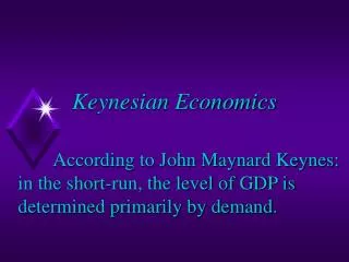
Aggregate Demand Theory Keynes’ General Theory Kaleckian alternative Aggregate Supply Function Relationship of firms’ expected sales receipts to level of employment hired Aggregate Demand Function Relationship of households’ expected purchases to level of employment Interaction produces Macreconomic equilibrium
Aggregate Supply and Demand • Keynes viewed Say’s Law as requiring a coincidence between the Z and D functions Source: Paul Davidson, “Reviving Keynes’ Revolution,” Why Economists Disagree, p. 70.
Keynes and Say’s Law Whether Keynes accurately portrayed Say’s Law has been a subject of a prolonged and ongoing debate. Leijonhufvud argues that what Say had in mind was a “constraint on reasoning,” and that therefore Say’s Law is really a relationship between plans and not the fruition of plans. We won’t enter into that debate here (take my Macroeconomics class in the spring if you want to understand the debate and its importance).
Aggregate Supply and Demand • Keynes argued that involuntary unemployment is due to a lack of effective demand (Given D at D’, equilibrium sales are E and employment is N1 rather than full employment Nf ‘ Source: Paul Davidson, “Reviving Keynes’ Revolution,” Why Economists Disagree, p. 70.
Aggregate Demand Theory The primary determinant of the level of effective demand is investment, which does not require saving. Rather investment only depends upon the willingness to borrow (tied to expected sales) and the willingness to lend (tied to expected sales). Thus the importance of consumer demand in molding the expectations of firms and banks to enter into loan contracts to finance investment.
Normative Criteria and Policy Espousal • Success at full employment and fair distribution of income rather than success at allocating resources • Government Management • Price and income policies can do good • Socialist to corporate liberalism