Download
1 / 40
400 likes | 477 Views
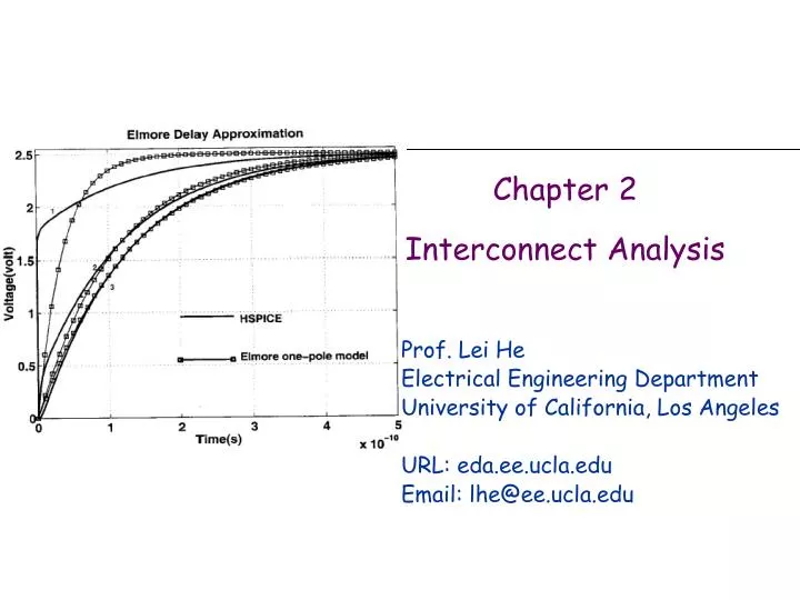
Chapter 2 Interconnect Analysis. Prof. Lei He Electrical Engineering Department University of California, Los Angeles URL: eda.ee.ucla.edu Email: lhe@ee.ucla.edu. Organization. Chapter 2a First/Second Order Analysis Chapter 2b Moment calculation and AWE

E N D
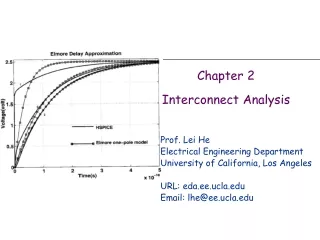
Chapter 2Interconnect Analysis Prof. Lei He Electrical Engineering Department University of California, Los Angeles URL: eda.ee.ucla.edu Email: lhe@ee.ucla.edu
Organization • Chapter 2a First/Second Order Analysis • Chapter 2b Moment calculation and AWE • Chapter 2c Projection based model order reduction
Projection Framework:Change of variables reduced state Note: q << N original state
Projection Framework • Original System • Substitute Note: now few variables (q<<N) in the state, but still thousands of equations (N)
Projection Framework (cont.) Reduction of number of equations: test multiplying by VqT If V and U biorthogonal
Projection Framework (cont.) qxn qxq nxn nxq
Approaches for picking V and U • Use Eigenvectors • Use Time Series Data • Compute • Use the SVD to pick q < k important vectors • Use Frequency Domain Data • Compute • Use the SVD to pick q < k important vectors • Use Krylov Subspace Vectors?
Intuitive view of Krylov subspace choice for change of base projection matrix Taylor series expansion: • change base and use only the first few vectors of the Taylor series expansion: equivalent to match first derivatives around expansion point U
Combine point and moment matching: multipoint moment matching • Multiple expansion points give larger band • Moment (derivates) matching gives more accurate • behavior in between expansion points
Aside on Krylov Subspaces - Definition The order k Krylov subspace generated from matrix A and vector b is defined as
Projection Framework: Moment Matching Theorem (E. Grimme 97) If and Then
Special simple case #1: expansion at s=0,V=U, orthonormal UTU=I If U and V are such that: Then the first q moments (derivatives) of the reduced system match
Need for Orthonormalization of U Vectors will line up with dominant eigenspace!
Need for Orthonormalization of U (cont.) • In "change of base matrix" U transforming to the new reduced state space, we can use ANY columns that span the reduced state space • In particular we can ORTHONORMALIZE the Krylov subspace vectors
For i = 1 to k Generates k+1 vectors! For j = 1 to i Orthogonalize new vector Normalize new vector Orthonormalization of U:The Arnoldi Algorithm
Special case #2: expansion at s=0, biorthogonal VTU=I If U and V are such that: Then the first 2q moments of reduced system match
PVL: Pade Via Lanczos[P. Feldmann, R. W. Freund TCAD95] • PVL is an implementation of the biorthogonal case 2: Use Lanczos process to biorthonormalize the columns of U and V: gives very good numerical stability
Case #3: Intuitive view of subspace choice for general expansion points • In stead of expanding around only s=0 we can expand around another points • For each expansion point the problem can then be put again in the standard form
s2 s1 s1=0 s3 Case #3: Intuitive view of Krylov subspace choice for general expansion points (cont.) Hence choosing Krylov subspace matches first kj of transfer function around each expansion point sj
Interconnected Systems • In reality, reduced models are only useful when connected together with other models and circuit elements in a composite simulation • Consider a state-space model connected to external circuitry (possibly with feedback!) ROM • Can we assure that the simulation of the composite system will be well-behaved? At least preclude non-physical behavior of the reduced model?
Passivity • Passive systems do not generate energy. We cannot extract out more energy than is stored. A passive system does not provideenergy that is not in its storage elements. • If the reduced model is not passive it can generate energy from nothingness and the simulation will explode
- - - - + + + + - - - - + + + + D D D D Q Q Q Q C C C C Interconnecting Passive Systems • The interconnection of stable models is not necessarily stable • BUT the interconnection of passive models is a passive model:
Sufficient conditions for passivity • Sufficient conditions for passivity: Note that these are NOT necessary conditions (common misconception)
Congruence Transformations Preserve Positive Semidefinitness • Def. congruence transformation same matrix • Note: case #1 in the projection framework V=U produces congruence transformations • Property: a congruence transformation preserves the positive semidefiniteness of the matrix • Proof. Just rename • Note:
PRIMA (for preserving passivity) (Odabasioglu, Celik, Pileggi TCAD98) A different implementation of case #1: V=U, UTU=I, Arnoldi Krylov Projection Framework: Use Arnoldi: Numerically very stable
PRIMA preserves passivity • The main difference between and case #1 and PRIMA: • case #1 applies the projection framework to • PRIMA applies the projection framework to • PRIMA preserves passivity because • uses Arnoldi so that U=V and the projection becomes a congruence transformation • E and A produced by electromagnetic analysis are typically positive semidefinite while may not be. • input matrix must be equal to output matrix
Homework 2 (due April 27) • (3) Modify the PRIMA code with single frequency expansion to multiple points expansion. You should use a vector fspan to pass the frequency expansion points. Compare the waveforms of the reduced model between the following two cases: • 1. Single point expansion at s=1e4. • 2. Four-point expansion at s=1e3, 1e5, 1e7, 1e9.
Format of the input matrices for test 1 1 19.4595 1.43391e-14 1 2 0.000464141 -2.9702e-15 1 3 -0.000542882 0.0 1 4 0.000152585 -7.5288e-15 1 5 0.000464074 -2.9702e-15 1 6 -0.000542801 0.0 1 68 -19.4595 0.0 2 1 0.0 -2.9702e-15 2 2 3.66672 2.44291e-13 2 3 0.0 -2.3594e-13 2 4 0.0 -5.3806e-15 2 72 -1.425 0.0 2 329 -2.06075 0.0 2 341 -0.091255 0.0 2 343 -0.0897199 0.0 3 1 -2.44188e-06 0.0 3 2 -0.000464141 -2.3594e-13 3 3 40.8898 2.42089e-13 …..
G,C,B,U,L matrices have been generated. Prima begins: Elapsed time is 2.003787 seconds. Prima done! Calculate original time domain response: Elapsed time is 2.868078 seconds. Original time domain response done! Calculate reduced time domain response: Elapsed time is 0.553771 seconds. Reduced time domain response done! Calculate original frequency response: Elapsed time is 1.192908 seconds. Original frequency response done! Calculate reduced frequency response: Elapsed time is 0.359126 seconds. Reduced frequency response done! Calculate original impulse response: Elapsed time is 0.052804 seconds. Original impulse response done! Calculate reduced impulse response: Elapsed time is 0.052701 seconds. Reduced impulse response done!