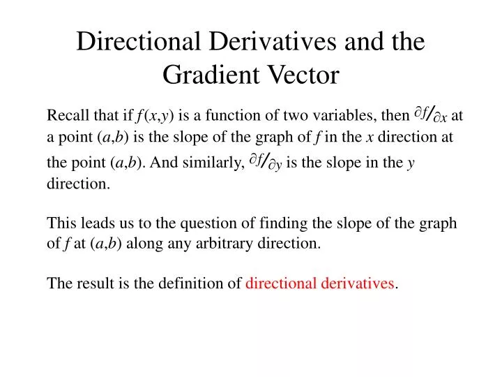
Directional Derivatives and the Gradient Vector

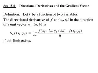
1. Directional Derivatives and the Gradient Vector Recall that if f(x,y) is a function of two variables, then f/x at a point (a,b) is the slope of the graph of f in the x direction at the point (a,b). And similarly, f/y is the slope in the y direction. This leads us to the question of finding the slope of the graph of f at (a,b) along any arbitrary direction. The result is the definition of directional derivatives.

2. North East Let’s pick a point P on this surface. Now imagine that we are passing through this point in the NE direction. To see the slope along this path at P, we cut the surface apart.

3. North East We can also travel along a perpendicular direction and the slope at the point P will be smaller (click).

4. North East We can also travel along a perpendicular direction and the slope at the point P will be smaller.

5. North East We can also travel along a perpendicular direction and the slope at the point P will be smaller.

6. Directional Derivatives Definition Suppose that f(x,y) is a function of two variables, and u = ,  is a unit vector, then the directional derivative of f at the point (x0,y0) along the direction of u is if the limit exists. Remark Since u is a unit vector on the xy-plane, it is more convenient to write u = cos, sin  where  is the angle between u and the positive x-axis (anticlockwise).

7. Directional Derivatives Remark Since u is a unit vector on the xy-plane, it is more convenient to write u = cos, sin  where  is the angle between u and the positive x-axis (anticlockwise). Using this notation, we have

8. Theorem If f(x,y) is differentiable at the point (x0,y0) and u = cos, sin  is a unit vector then Definition If f(x,y) is a function of two variables x and y, then the gradient of f is the vector function f defined by

9. More General Cases If f(x,y,z) is a differentiable function of three variables, and u is a unit vector in 3D, then the directional derivative of f at any point within the domain of f is Duf(x,y,z) = f(x,y,z) · u

10. Significance of the Gradient Vector Theorem If f(x,y) is a differentiable function of two variables, then (1) the direction of f(x,y) is the direction along which the directional derivative of fat (x,y) is the greatest. In other words, the graph of f at (x,y) has the greatest slope in the direction of f(x,y). (2) the magnitude | f(x,y)| is the maximal value of the slope of (the graph of) f at the point (x,y). Remark The above theorem also applies to functions of 3 variables.

11. A Geometrical Picture At any point (x0,y0) in the domain of f, if u is a unit vector along the direction of the tangent to the level curve f(x,y) = f (x0,y0), then Duf(x0,y0) = 0 Consequently, the gradient vector f at any point (x0,y0) must be perpendicular to the (tangent of the) level curve at (x0,y0). level curve f

12. Example:

13. y x

14. Special Application in 3D If we extend the previous result to 3D, the gradient vector f at any point (x0,y0,z0) must be perpendicular to the level surface of f through the point (x0,y0,z0, f(x0,y0,z0)). Consequently, f will be a normal of the tangent plane to the level surface at (x0,y0,z0), and we can use this information to construct an equation of that tangent plane. (Fortunately, this is not a popular question in this course.)

15. Maximum and Minimum Values Absolute max local max absolute min local min

16. It is clear that if the function is differentiable, then at any local maximum or minimum the tangent plane must be horizontal. This means that both partial derivatives must be zero at that point (x0,y0), or in other words, f(x0,y0) =0 • Definition: • If fis a function of several variables, then we say that P (in the domain of f ) is a critical point of fif either • at least one partial derivative of f does not exist at P, or • f = 0 at P.

17. Definitions A function f(x,y) is said to have a local maximum at the point (a,b) if there is a small neighborhood U of (a, b), such that f(a, b) ≥f(x, y) for every (x, y) in U. A function f(x,y) is said to have a strictlocal maximum at the point (a,b) if there is a small neighborhood U of (a, b), such that f(a, b) >f(x, y) for every (x, y) in U – {(a, b)}

18. Local Maximum and Local Minimum A function f(x,y) is said to have a local minimum at the point (a,b) if there is a small neighborhood U of (a, b), such that f(a, b) ≤f(x, y) for every (x, y) in U. A function f(x,y) is said to have a strictlocal minimum at the point (a,b) if there is a small neighborhood U of (a, b), such that f(a, b) <f(x, y) for every (x, y) in U – {(a, b)}

19. Local Maximum and Local Minimum A function f(x, y) is said to have a saddle point at (a, b) if it has a critical point at (a,b) and if in every small neighborhood U of (a,b), we can find two points (x1, y1) and (x2, y2) such that f(a, b) < f(x1, y2) and f(a, b) > f(x1, y2)

20. Example of a Saddle point If we cut the surface along the x-axis, we see that the blinking point appears to be a local maximum. But if we cut the surface along the y-axis, we see that the blinking point appears to be a local minimum. (click)

21. But if we cut the surface along the y-axis, we see that the blinking point appears to be a local minimum.

22. But if we cut the surface along the y-axis, we see that the blinking point appears to be a local minimum. This critical point is called a saddle point.

23. 2 1 0 -1 -2 -1 -2 -0.5 -1 0 0.5 0 1 1 1.5 2 2 A monkey saddle f (x, y) = 6xy2 – 2x3 – 3y4

24. How can we use partial derivatives to determine whether a critical point is a local minimum? If both can we say that (a,b) is a local minimum?

25. 0.1 0 -0.1 -0.2 -1 -0.3 -0.5 -1 0 -0.5 0 0.5 0.5 1 1 How can we use partial derivatives to determine whether a critical point is a local maximum?

26. Second Derivative Test Suppose that (a,b) is a critical point for f and all second partial derivatives of fare continuous on a disk with center (a,b) and let • Then • f(a,b) is a strict local minimum if D > 0 and 2f/x2(a,b) > 0 • f(a,b) is a strict local maximum if D > 0 and 2f/x2(a,b) < 0 • (a,b) is a saddle point for f if D < 0, • the test is inconclusive if D = 0.

27. 1 0.8 0.6 0.4 0.2 0 -2 -1 2 0 1 x 0 1 y -1 2 -2 Example Find all critical points of the following function and use the 2nd Partial Derivative test to determine the nature of each critical point.

28. Second Derivative Test(for functions of 3 variables) Suppose that (a,b,c) is a critical point for f and all second partial derivatives of fare continuous on a disk with center (a,b,c) and let

29. Then • f(a,b,c) is a strict local minimum if D1 > 0, D2 > 0 and D3 > 0 • f(a,b,c) is a strict local maximum if D1 < 0, D2 > 0 and D3 < 0 • (a,b,c) is a saddle point for f if D2 < 0, • in all other cases, the test is inconclusive.

30. Special Example This example shows that f can have a local minimum at (0,0) even if D(0,0) = 0. Let f(x,y) = x4y4, then Clearly all these functions are 0 at (0,0), hence D(0,0) = 0, but we can easily see from the graph that (0,0) is an absolute min.

31. Extremum with Constraint Suppose that f(x,y) is a function of two variables. We want to find the maximum (or minimum) of f with the restriction that (x,y) must also satisfy the condition that g(x,y) = k for some given function g(x,y) and a given number k.

32. Extremum with constraint

33. Extremum with constraint The yellow curve is the set of points {(x, y, f(x,y) : g(x,y) = k}

34. Extremum with constraint The green curve is a level curve on the surface that meets the highest point of the yellow curve. The yellow curve is the set of points {(x, y, f(x,y) : g(x,y) = k}

35. g(x,y) = k level curve of f P(x0, y0) If we project these two curves down to the xy-plane, they would look like where P(x0,y0) is the point where the curve attains its max. Case 1: f(x0,y0) ≠0 This means that P(x0,y0) is not a critical point for f , and the vector f(x0,y0) must be pointing perpendicular to the level curve of f at this point. Moreover, the curve g(x, y) = k must be tangential to the level curve of f at this point P in order to achieve a local max (or min).

36. g(x,y) = k level curve of f P(x0, y0) If in addition, it also happens that g(x0,y0) ≠0 (but this is almost always the case, see remarks at the end.), then g(x0,y0) must also be perpendicular to the curve g(x,y) = k at (x0,y0). This means that f(x0,y0) is parallel to g(x0,y0) and hence for some real number λ.

37. g(x,y) = k level curve of f P(x0, y0) Remark: If g(x0,y0) = 0, then (x0,y0) would be a critical point for g, and hence the curve g(x, y) = k would degenerate into a single point at (x0,y0), or it crosses itself at this point. Fortunately these cases are rare. Case 2: f(x0,y0) =0 In this case, clearly f(x0,y0) = 0 g(x0,y0) . Hence it is also true that for some real number λ.

38. Lagrange Multipliers Theorem Suppose that f(x,y) and g(x,y) are both differentiable functions and P(x0,y0) is local extremum of funder the constraint g(x,y) = k. If g(x0,y0) ≠0, then there is a real number λ such that Remark: This theorem also works for functions of more than 2 variables, such as

39. Method of Lagrange Multipliers • To find the maximum and minimum values of the function f(x,y,z) subject to the constraint g(x, y, z) = k (assuming that theseextreme values exist): • (a) Check that g(x, y, z) will not be 0 on the curve. • Find all values of x, y, z, and λsuch thatf(x, y, z) =λ g(x, y, z) andg(x, y, z) = k • Evaluate fat all the points (x, y, z) obtained from step (a). The largest of these is the maximum and the least is the minimum.

40. 4 y 2 x 0 -3 -2 -1 1 2 3 -2 -4 Example Find the maximum and minimum values of f(x,y) = 4xy, subject to the constraint 16x2 – 8xy + 9y2 = 144. Solution: First we let g(x, y) = 16x2 – 8xy + 9y2 We then observe that the “graph” of the constraint is an ellipse with non-horizontal and non-vertical axes. g = 32x – 8y, -8x + 18y and g = 0 if and only if (x, y) = (0, 0), which will not occur on the curve because it does not pass through the origin.

41. f = 4y, 4x and f = λg implies that 4y = λ(32x – 8y) ---------- (1) 4x = λ(-8x + 18y) ---------- (2) y = λ(8x – 2y) ---------- (1) 2x = λ(-4x + 9y) ---------- (2)

42. Combining the above two, we have But x cannot be zero, because otherwise y = 0, and (0, 0) is not a point on the ellipse. Therefore we must have i.e. 72 λ2 = (4 λ +2)(2 λ +1) giving λ =¼ or − 1/8 If λ = ¼ , then y = 4x/3 and If λ = − 1/8 , then y = -4x/3 and