Download
1 / 19
210 likes | 351 Views
Introduction to Experience Rating. Joy Takahashi - American Re Broker Market CAS Ratemaking Seminar Session REI-39 March 7, 2002 Tampa, FL. Introduction to Experience Rating. Classical Burning Cost Method Frequency Based Method. Classical Burning Cost Method Basic Steps.

E N D
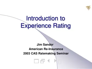
Introduction to Experience Rating Joy Takahashi - American Re Broker Market CAS Ratemaking Seminar Session REI-39 March 7, 2002 Tampa, FL
Introduction to Experience Rating Classical Burning Cost Method Frequency Based Method
Classical Burning Cost MethodBasic Steps • Obtain large loss listing and calculate nominal excess losses in layer (i.e. 100k xs 100k). • Apply trend factors; cap at policy limits. • Apply loss development factors. • Divide losses by adjusted subject premium to derive an expected loss cost.
Classical Burning CostStep 1 - Collect data Log AY Rptd Loss Pol Limit Loss in Layer 1 97 255,692 300,000 100,000 5 97 75,324 0 6 97 130,235 100,000 0 14 98 1,152,028 1,000,000 100,000 19 99 175,274 75,274 38 01 360,044 1,000,000 100,000 Total 5,747,914 997,631 Note: Losses include ALAE. Not all losses are displayed.
Classical Burning CostStep 2 - Trend Trend Trended Policy Loss in Log AY Factor Loss Limit Layer 1 97 1.338 342,174 300,000 100,000 5 97 1.338 100,801 801 6 97 1.338 174,284 100,000 0 14 98 1.262 1,454,409 1,000,000 100,000 19 99 1.191 208,754 100,000 38 01 1.060 381,647 1,000,000 100,000 Total 6,907,025 1,234,012 Total w/ freq trend 1,312,100
Classical Burning CostStep 3 - Loss Development Trended XS Ultimate AY Loss in Layer LDF Loss in Layer 97 251,500 1.238 311,300 98 300,100 1.485 445,600 99 212,200 2.302 488,500 00 442,700 4.604 2,038,100 01 105,500 41.432 4,370,300 Total 1,312,100 7,653,800
Classical Burning CostStep 4 - Divide by Subject Premium Nominal Trended Tr & Dev AY Adj SEP $ % $ % $ % 97 12,763 144.4 1.1% 251.5 2.0% 311.3 2.4% 98 18,233 215.5 1.2% 300.1 1.6% 445.6 2.4% 99 23,133 175.3 0.8% 212.2 0.9% 488.5 2.1% 00 26,460 362.5 1.4% 442.7 1.7% 2,038.1 7.7% 01 31,500 100.0 0.3% 105.5 0.3% 4,370.3 13.9% Est ‘02 40,000 400.8 1.0% 533.6 1.3% 967.5 2.4%
Classical Burning CostPotential Problems • Presence or absence of a few large claims drives the indicated rates. • Order of application of development, trend and capping makes a difference. • Trending individual claims past policy limits. • Impact of current policy limit profile vs. historicals. • History not reflective of current situation: reserving practices, type of business, coverage, etc.
Frequency Based MethodBasic Steps • Estimate # of claims above a data limit (e.g. 28 claims > $50,000). • Use size of loss curves to project # of claims above the retention (e.g. 14.4 claims > $100,000 retention). • Distribute the projected counts by policy limit; eliminate counts with policy limit below retention (e.g. 12.25 claims if 15% of exposure has $100,000 limits). • Use size of loss curves to project average severity of claims in layer (e.g. $69,495 sev. in 100 x 100 layer). • Multiply frequency by severity to get total losses. • Divide by adjusted subject premium to get expected loss cost.
Frequency BasedStep 1 - Project # of Claims Above Data Limit Detrended Actual Freq Clm Cnt Projected AY Data Limit # > DDL Trend Dev Fctr # > DL 97 37,363 6 1.104 1.050 6.96 98 39,605 8 1.082 1.155 10.00 99 41,981 5 1.061 1.559 8.27 00 44,500 13 1.040 2.339 31.63 01 47,170 5 1.020 5.847 29.82 Selected 50,000 28.00
Frequency BasedStep 1a - Selection Process Projected Projected AY # > DL Adj SEP Frequency # @ 02 Levels 97 6.96 12,763 .545 21.8 98 10.00 18,233 .549 21.9 99 8.27 23,153 .357 14.3 00 31.63 26,460 1.196 47.8 01 29.82 31,500 .947 37.9 Selected 40,000 .700 28.00
Frequency BasedStep 2 - Project # of Claims Above Retention Projected Limit Retention # > Ret. 50,000 xs 50,000 28.00 100,000 xs 100,000 14.41 * 300,000 xs 200,000 7.22 * 500,000 xs 500,000 2.84 * * Note: these were derived from pareto size-of-loss curve frequency formula: N X [(DL + B)/(R + B)] ^ Q
Frequency BasedStep 3 - Include Impact of Policy Limits Projected # Clms by Pol Limit New Limit Retention # > Ret 100 300 500 1MM # > Ret 50,000 50,000 28.00 4.20 5.60 7.00 11.20 28.00 100,000 100,000 14.41 2.16 2.88 3.60 5.76 12.25 300,000 200,000 7.22 1.08 1.44 1.81 2.89 6.14 500,000 500,000 2.84 .43 .57 .71 1.14 1.14 ‘02 Policy Limit Distribution: 15% 20% 25% 40% Note: Claims below line are eliminated from the layer due to policy limits.
Frequency BasedStep 4 - Estimate Loss $ in Layer Projected Avg Sev. Loss Cost Limit Retention # > Ret. in Layer in Layer 100,000 100,000 14.41 69,495 1,001,423 100,000 100,000 12.25 69,495 851,210 Note: Average severities are from pareto size-of-loss curve severity formula: [(R+B)/(Q-1)] X {1 - [(R+B)/(R+L+B)]^(Q-1)}
Frequency Based MethodStep 5 - Divide by Subject Premium Subject Selected Loss Cost Earned Prem. $ % 40,000,000 851,210 2.1%
Frequency Based MethodPotential Problems • Credibility of claim count development factors • Adjustment of development factors by data limit • Picking an appropriate data limit • Testing of size-of-loss assumptions
Frequency Based MethodAdvanced Techniques Goal: Fitting individual claim data to size-of-loss curve. • Trend individual claims to common accident date. • Develop trended individual claims to ultimate, using report year development factors if available. • Fit developed and trended claims to size-of-loss curve. • Test curve with actual data and industry curves. • Use new fitted curve in frequency based method to derive new loss cost.
Frequency Based MethodAdvanced Techniques Comparison of Actual and Fitted Average Severities (in 000’s)
Experience RatingComparison of Methods Classical Burning CostOriginalAlternative Est. Losses $ 1,089,100 967,500 Est. Loss Cost % 2.7% 2.4% Frequency Based MtdOriginalCo. Fitted Est. Losses $ 851,210 955,118 Est. Loss Cost % 2.1% 2.4% Selected1,000,000 2.5%