Download
1 / 26
260 likes | 265 Views
UNIT 6 Pricing under different market structures. Perfect Competition. Market Structure. Pure Monopoly. Perfect Competition. Monopolistic Competition. Oligopoly. Duopoly. Monopoly. The further right on the scale, the greater the degree of monopoly power exercised by the firm.

E N D
UNIT 6Pricing under different market structures Perfect Competition
Market Structure Pure Monopoly Perfect Competition Monopolistic Competition Oligopoly Duopoly Monopoly The further right on the scale, the greater the degree of monopoly power exercised by the firm.
Perfect Competition Firms are price-takers Each produces only a very small portion of total market or industry output All firms produce a homogeneous product Entry into & exit from the market is unrestricted
Demand for a Competitive Price-Taker Demand curve is horizontal at price determined by intersection of market demand & supply Perfectly elastic Marginal revenue equals price Demand curve is also marginal revenue curve (D = MR) Can sell all they want at the market price Each additional unit of sales adds to total revenue an amount equal to price
Demand for a Competitive Price-Taking Firm S P0 P0 D = MR D Q0 Price (dollars) Price (dollars) 0 0 Quantity Quantity Panel B – Demand curve facing a price-taker Panel A – Market
Short-Run Market Supply and Demand Graph P Market P Firm MC Market Supply ATC P P P = D = MR Profits ATC Market Demand Q Q Qprofit max 14-6
Profit-Maximization in the Short Run In the short run, managers must make two decisions: Produce or shut down? If shut down, produce no output and hire no variable inputs If shut down, firm loses amount equal to TFC If produce, what is the optimal output level? If firm does produce, then how much? Produce amount that maximizes economic profit Profit =
Determining Profits Graphically: A Firm with Profit P Find output where MC = MR, this is the profit maximizing Q MC MC = MR ATC Find profit per unit where the profit max Q intersects ATC P = D = MR P Profits AVC ATC ATC at Qprofit max Since P>ATC at the profit maximizing quantity, this firm is earning profits Q Qprofit max 14-8
Determining Profits Graphically: A Firm with Losses P Find output where MC = MR, this is the profit maximizing Q MC ATC ATC at Qprofit max Find profit per unit where the profit max Q intersects ATC AVC ATC P = D = MR Losses P Since P<ATC at the profit maximizing quantity, this firm is earning losses MC = MR Q Qprofit max 14-9
Determining Profits Graphically: A Firm with Zero Profit or Losses P Find output where MC = MR, this is the profit maximizing Q MC ATC Find profit per unit where the profit max Q intersects ATC MC = MR AVC P = D = MR P =ATC ATC at Qprofit max Since P=ATC at the profit maximizing quantity, this firm is earning zero profit or loss Q Qprofit max 14-10
Determining Profits Graphically: The Shutdown Decision • The shutdown point is the point below which the firm will be better off if it shuts down than it will if it stays in business • If P>min of AVC, then the firm will still produce, but earn a loss • If P<min of AVC, the firm will shut down • If a firm shuts down, it still has to pay its fixed costs P MC ATC AVC P = D = MR PShutdown Q Qprofit max 14-11
Short-Run Output Decision Firm’s manager will produce output where P = MC as long as: TR TVC or, equivalently, P AVC If price is less than average variable cost (P AVC), manager will shut down Produce zero output Lose only total fixed costs Shutdown price is minimum AVC
Irrelevance of Fixed Costs Fixed costs are irrelevant in the production decision Level of fixed cost has no effect on marginal cost or minimum average variable cost Thus no effect on optimal level of output
The Competitive Firm’s Short run Supply • Portion of MC curve above AVCmin • MC curve gives the relationship between P and Qs P MC ATC AVC P = D = MR PShutdown Q Qprofit max 14-14
The number of firms in the industry The average size of firms in the industry measured by quantity of fixed inputs employed The price of variable inputs used by firms in the industry The technology employed in the industry. Determinants of Market Supply
AVC tells whether to produce Shut down if price falls below minimum AVC SMC tells how much to produce If P minimum AVC, produce output at which P = SMC ATC tells how much profit/loss if produce Summary of Short-Run Output Decision •
Long-Run Competitive Equilibrium All firms are in profit-maximizing equilibrium (P = LMC) Occurs because of entry/exit of firms in/out of industry Market adjusts so P = LMC = LAC
Long-Run Competitive Equilibrium P • Market adjusts so • P = LMC = LAC LMC Since P=LAC at the profit maximizing quantity, this firm is earning zero profit LAC MC = MR P = D = MR P =LAC ATC at Qprofit max Q Qprofit max 14-20
LAC and LMC • Long-run Average Cost (LAC) curve • is U-shaped. • the envelope of all the short-run average cost curves; • driven by economies and diseconomies of scale. • Long-run Marginal Cost (LMC) curve • Also U-shaped; • intersects LAC at LAC’s minimum point.
Economies and Diseconomies of Scale • Economies of Scale- long run average cost decreases as output increases. • Technological factors • Specialization • Diseconomies of Scale: - long run average cost increases as output increases. • Problems with management – becomes costly, unwieldy
COST LAC SAC1 SAC2 Diseconomies of Scale Economies of Scale 0 Q Q1 LONG-RUN AVERAGE COST CURVE
LONG-RUN AVERAGE and MARGINAL COST CURVES LMC COST LAC 0 Q Q1
In a given market, demand is described by the equation QD = 1,800 - 10P and supply is described by QS = 200 + 10P. Determine the equilibrium price and quantity. The marginal cost of a firm under perfect competition is given by the equation MC = 20 + 2QF. The market price is $50 per unit. Determine the firm’s profit-maximizing level of output. For a perfectly competitive firm, long-run average cost is: LAC = 300 - 20QF + 0.5QF2., where QF denotes the firm’s output. Determine the firm’s long-run profit-maximizing output and price. Class Exercise
Setting QD = QS implies P = $80 and Q = 1,000 units. 2. The firm maximizes its profit by setting: P = MC. Therefore, we have 50 = 20 + 2QF, or QF = 15. 3. In the long run, under perfect competition, firms will produce at the minimum point on their LAC curve. To find the minimum of LAC, we set dLAC/dQ equal to 0. Therefore, -20 + QF = 0, so that QF = 20. The firm’s demand curve is horizontal and tangent to LAC. Therefore, price is equal to the minimum value of LAC. We find minimum LAC to be: 300 - (20)(20) +0.5(20)² = 100. Thus, PC = 100. Class Exercise Solved