Download
1 / 23
230 likes | 390 Views
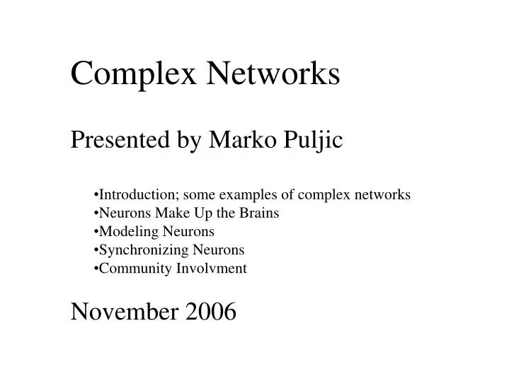
Complex Networks Presented by Marko Puljic Introduction; some examples of complex networks Neurons Make Up the Brains Modeling Neurons Synchronizing Neurons Community Involvment November 2006. Introduction. Complex weblike structures (couple examples)

E N D
Complex Networks • Presented by Marko Puljic • Introduction; some examples of complex networks • Neurons Make Up the Brains • Modeling Neurons • Synchronizing Neurons • Community Involvment • November 2006
Introduction Complex weblike structures (couple examples) • cell is best described as a complex network of chemicals connected by chemical reactions; • internetis a complex network of routers and computers linked by various physical or wireless links; • social network / human beings with edges representing • various social relationships; • world wide web is an virtual network of Web pages connected by hyperlinks.
Introduction Complex system has many interacting components (1011 neurons, 104 types of proteins, 106 routers, 109 web pages) with not obvious aggregate behaviour. (assembling of the many results in something unexpected) Networks in complex systems who interacts with whom • networks - collection of evolving components connected • cellular automata - Von Neumann network, Conway, Wolfram • physicists assumed perfect knowledge of individual-level properties • social networks by Watts, Strogatz, Barabasi, Kleinberg
Introduction Advances in complex networks prompted by • computerization of data acquisition • increased computing power • breakdown of boundaries between disciplines • need to move beyond reductionist approaches and try to understand the behavior of the system as a whole • Concepts / Measures • Small worlds: short path between any two nodes in the network. • Clustering: cliques, e.g. circles of friends in which every member knows every other member. • Degree distribution: number of edges per node. P(‘k’), which gives the probability that a randomly selected node has exactly ‘k’ edges.
From Y. Tu, “How robust is the Internet?” , Nature 406, 353 (2000) Internet
Introduction Hierarchy of bio-networks • Metabolic network: production of necessary chemical compounds • Binding network: enzymes bind to their substrates in a metabolic network and to other proteins to form complexes • Regulatory network: turns on and off particular groups of proteins in response to signals • HIGHER LEVELS: cell-to cell communication (e.g. neurons in a brain), food webs, social networks, etc.
Single-celled eukaryote:S. cerevisiae Transcription regulatory networks Prokaryotic bacterium:E. coli
Neurons Make Up the Brains INSPIRATION FROM NEURONAL ARCHITECTURE schematic view of axon Neuropil: Densely connected filamentous texture of nervous tissue + mesoscopic state variables are describe by the collective activities of neurons in the pulse and wave modes. Transformation of the neurons from one mode of existence to another is example of state transition. + microscopic state variables are described by the activity of the single neuron, which converts incoming pulses to waves, sums them, converts its integrated wave to a pulse train, and transmits that train to all its axonal branches.
Neurons Make Up the Brains biologically motivated mathematical theory of neuropercolation • explaining the spatial-temporal characteristics of phase transitions in a neural network model • describe dynamical behavior of the neuropil in cortices • used for the interpretation of the operation of dynamical memories in artificial and biological systems • understanding of information encoding in the central nervous system • implement these principles in a new generation of computational devices
Modeling Neurons MODEL WITH NON-LOCAL CONNECTIONS Assignment of Neighbors site with local neighbors only site with additional remote neighbor NxN Lattice/Torus 1) every site has 4 local neighbors with same relative position 2) randomly selected sites with the additional remote neighbor 3) one way directions for remote neighbor 4) once assigned neighbors never change Site activation changes in time, which is measured in discrete steps. At each step activation is defined by the transition rules, (see next).
Modeling Neurons Transition Rules step i єε 1-єε .5 єε ε .5 1-єε step i+1 (c) (b) (a) } { є; if majority active 1-є; if majority inactive 0.5; if number of inactive = number of active є; if majority inactive neighbors 1-є; if majority active 0.5; if number of inactive = number of active chance of being inactive = { } chance of being active=
Modeling Neurons Phase Transitions in Local Random Percolation • Varying p: • Obtain phase transition • similar to Ising models • Two stable states: • With high and low density • In large lattice one dominates • If p is close to critical value: • Two states coexist for long є close to critical probability
Modeling Neurons Critical ε vs. Remote Connections • Adding neighbors and/or changing the connection architecture changes the critical ε with lower and upper bound when the lattice has no remote neighbors and when lattice is fully connected respectively. • It is possible to simulate critical ε between lower (0.13428) and upper bound (0.233) to any desired precision by arbitrary lattice size and connection architecture. *100 corresponds to 400 remote neighbors, 20 to 80 remote neighbors and so on.
Modeling Neurons Density and Clusters Cluster is constituted of the sites that have same activation value, which are connected in the network through their local neighborhood. example: Inactive clusters of size 4, 3, 5, 17, and 2 in shaded region, respectively.
Synchronizing Neurons Chaotic Itinerancy I. Tsuda:"In low-dimensional dynamical systems, the [asymptotic] dynamical behavior is classified into four categories: a steady state , a periodic state , a quasi-periodic state, and a chaotic state . Each class of behavior is represented by a fixed point attractor, a limit cycle, a torus, and a strange attractor, respectively. However, the complex behavior in high-dimensional dynamical systems is not always described by these attractors. A more ordered but more complex behavior than these types of behavior often appears. We [Kaneko, Tsuda et al.] have found one such universal behavior in non-equilibrium neural networks, globally coupled chaotic systems, and optical delayed systems. We called it a chaotic itinerancy. “ "Chaotic itinerancy (CI) is considered as a novel universal class of dynamics with large degrees of freedom. In CI, an orbit successively itinerates over (quasi-) attractors which have effectively small degrees of freedom.” Figure: Schematic drawing of chaotic itinerancy. Dynamical orbits are attracted to a certain attractor ruin, but they leave via an unstable manifold after a (short or long) stay around it and move toward another attractor ruin. This successive chaotic transition continues unless a strong input is received. An attractor ruin is a destabilized Milnor attractor, which can be a fixed point, a limit cycle, a torus or a strange attractor that possesses unstable directions.
Chaotic Itinerancy The difference between transitions created by producing chaotic itinerancy and by introducing noise. (a) A transition created by introducing external noise. If the noise amplitude is small, the probability of transition is small. Then, one may try to increase the noise level in order to increase the chance of a transition. But this effort is not effective because the probability of the same state recovering is also increased as the noise level increases. In order to avoid this difficulty, one may adopt a simulated annealing method, which is equivalent to using an "intelligent" noise whose amplitude decreases just when the state transition begins. (b) A transition created by producing chaotic itinerancy. In each subsystem, dynamical orbits are absorbed into a basin of a certain attractor, where an attractor can be a fixed point, a limit cycle, a torus, or a strange attractor. The instability along a direction normal to such a subspace insures a transition from one Milnor attractor ruin to another. The transition is autonomous.
00 01 .. .. .. 77 00 01 .. .. .. 77 Synchronizing Neurons Experiments on the Lattices Objective: locate epochs of synchrony & stable spatial patterns using 64 channels that divide the lattice. find the correlations among the channels and ratios of variances of the channel activations and the system’s activation as a whole. Measurements Used: varc( di ) = E[ ( di – di-average )2 ]; variance of the channel i, vars( d ) = E[ ( d – daverage )2 ]; variance of the system, ratio as a measure of synchrony when the covariance is high = varc/ vars; Lattice/Torus channel activation at time t channel 00 . channel activation at time t+n channel 63 (covers 256 sites)
Synchronizing Neurons 'Local' Systems with є << єc and System with є > єc • low correlation • no spatial patterns • correlation coefficient of 50% • no spatial patterns
Synchronizing Neurons System With 100% of Four Remote Connections - Near єc Coupled lattices: http://cnd.memphis.edu/neuropercolation/presentation/polarized.shtml http://cnd.memphis.edu/neuropercolation/presentation/CRCAsync6.shtml
Community Involvements the University of Memphis Center for Information Assurance • Computer Science Department in collaboration • Management of Information Systems • Cecil C. Humphreys School of Law • Department of Criminology and Criminal Justice • Electrical and Computer Engineering • U of M Information Technology Division Center for IA is dedicated to providing world-class research, training, and career development for Information Assurance professionals and students alike by organizing community events, special purpose conferences, and vendor specific training programs. http://www.cs.memphis.edu/~dasgupta/
References J. von Neumann, “Theory of Self-Reproducing Automata," (Ed. by A. W. Burks), Univ. of Illinois Press, Champaign, (1966) S. Wolfram, "Cellular Automata and Complexity: Collected Papers," Addison-Wesley, Reading MA, (1994) W. J. Freeman, ``How Brains Make Up Their Minds,'' Columbia University Press, New York (1999) K. Kaneko, I. Tsuda, ``Chaotic Itinerancy,'' Chaos, 13 926-936 (2003) K. Kaneko, I. Tsuda, ``Chaotic Itinerancy,'' Chaos, 13 926-936 (2003) M. Puljic, PhD Dissertation, “Neuropercolation”