Download

1 / 36
360 likes | 381 Views
Planar Orientations. Chapter 4 (4.1-4.6) in the book Written By: Tomer Heber. Outline & Goal. In this lesson we will deal with planar st-graphs (which will be explained later on). We will review several algorithms for representing a st-planar graph.

E N D
Planar Orientations Chapter 4 (4.1-4.6) in the book Written By: Tomer Heber
Outline & Goal • In this lesson we will deal with planar st-graphs (which will be explained later on). • We will review several algorithms for representing a st-planar graph. • We will also learn that by using those representations we can turn a st-planar graph, to a more specific shape (such as a polyline). The goal of this lesson is simple: Which is to learn of ways to represent a st-graph in a more “useful” and “aesthetic” representation.
Numbering of Digraphs • A topological numbering of G is an assignment of numbers to the vertices of G, such that, for every edge (u,v) of G, the number assigned to v is greater then the one assigned to u. 5 2 3 4 2 1
Numbering of Digraphs (2) • A topological sorting is a topological numbering of G, such that every vertex is assigned a distinct integer between 1 and n. • A topological sorting is unique if G has a directed path that visits every vertex. 6 5 3 4 2 1
Numbering of Digraphs (3) • The following statements are equivalent: • G is acyclic. • G admits a topological numbering. • G admits a topological sorting. In other words a topological numbering (sorting) can be done only on an acyclic graph.
Planar Graph • A planar graph is a graph which can be embedded in the plane, i.e., it can be drawn on the plane in such a way that its edges intersect only at their endpoints. Faces
ST-Graph • An acyclic digraph with a single source s and a single sink t is called an st-graph. Sink “t” has no outgoing edges! t s Source “s” has no incoming edges!
ST-Graph (2) • Let G be an st-graph. The following simple properties hold: • Given a topological numbering of G. every directed path of G visits with increasing numbers. • For every vertex v of G, there exists a simple directed path from s (source) to t (sink) that contains v.
Planar ST-Graph • A planar st-graph is an st-graph that is planar and embedded with vertices s and t on the boundary of the external face. t s
Planar ST-Graph (2) • Let G be a planer st-graph and F be its set of faces. We conventionally assume that F contains two representatives for the external face: • The “left external face” s* • The “right external face” t* s* t*
Planar ST-Graph (3) • For each edge e = (u,v), we define orig(e) = u and dest(e) = v. • We define left(e) (resp. right(e)) to be the face to the left (resp. right) of e. dest(e) = v v orig(e) = u f1 left(e) = f1 e u left(e) = f2 f2
Planar ST-Graph Properties • Lemma 1:Each face f of G consists of two directed paths with common origin called orig(f), and common destination called dest(f). • Proof: Let f be a face of G for which the lemma is not true. t dest(f) There must be a path from vertex u to the “sink” t w Since the graph is planar there must be a node where the passes intersect We receive a cycle! u There must be a path from the “source” s to vertex w orig(f) s
Planar ST-Graph Properties (2) • Lemma 2: The incoming edges for each vertex of G appear consecutively around v, and so do the outgoing edges. • Proof: The lemma holds trivially for the vertices s and t. Let v be any other vertex, and suppose for a contradiction, that there are edges (v,w0), (w1,v), (v,w2), (w3,v). t w0 w1 We now have a cycle! v x w2 w3 s Because every vertex in a st-graph has a simple path from “s” to “t” we add the following paths… Because the graph is planar we add the vertex “x” to the graph.
Planar ST-Graph Properties (3) • Since the incoming (outgoing) edges of each vertex of G appear consecutively we define the face separating the incoming edges from the outgoing edges in clockwise order, left(v), and the other separating face is called right(v).
Planar ST-Graph G* • We define a digraph G* associated with planar st-graph G, as follows: • The vertex set of G* is the set F of faces (recall that F has two representatives, s* and t*, of the external face. • For every edge e != (s,t) of G, G* has an e* = (f,g) where f = left(e) and g = right(e). left(e) e right(e) Notice that G* is a planar st-graph as well
Lemma 3 • An element of is called an object of planar st-graph G. • For vertex v, we define orig(v) = dest(v) = v. • For a face f, we define left(f) = right(f) = f. * Reminder we have already defined previously: left(v), right(v), left(e), right(e), orig(e), dest(e), orig(f) and dest(f).
Lemma 3 (2) • Lemma 3: For any two objects o1 and o2 of a planar st-graph G, exactlyone of the following holds: • G has a directed path from dest(o1) to orig(o2). • G has a directed path from dest(o2) to orig(o1). • G* has a directed path from right(o1) to left(o2). • G* has a directed path from right(o2) to left(o2).
Tile • A tile is a rectangle with sides parallel to the coordinate axes. • A tilecan be unbounded or can degenerate to a segment or a point. • Two tiles are horizontally (vertically) adjacent if they share a portion of a vertical (horizontal) side. Tiles: Vertically adjacent:
Tessellation Representation • Let G be a planar st-graph. A tessellation representation Θ for G maps each object o of G into a tile Θ(o) such that: • The interiors of tiles Θ(o1) and Θ(o2) are disjoint whenever o1 != o2. • The union of all tiles Θ(o), is a rectangle. • Tiles Θ(o1) and Θ(o2) are horizontally adjacent if and only if o1 = left(o2) or o1 = right(o2) or o2 = left(o1) or o2 = right(o1). • Tiles Θ(o1) and Θ(o2) are vertically adjacent if and only if o1 = orig(o2) or o1 = dest(o2) or o2 = orig(o1) or o2 = dest(o1).
Tessellation Representation (2) 4 3 1 f 4 3 3 2 4 X(left(e)) = 0 X(left(f)) = 3 2 0 2 X(right(e)) = 1 X(right(f)) = 3 2 1 Y(orig(e)) = 0 Y(orig(f)) = 2 Y(dest(e)) = 2 Y(dest(f)) = 4 1 3 e 1 1 0 0 0 1 2 3 4
Tessellation Representation (3) • The correctness of the algorithm is based on Lemma 3: • Let there be tile t1 and tile t2, from Lemma 3 t1 is either: above t2, below t2, left of t2 or right of t2. And only one of this directions is true. • Since each line of the algorithm is O(n), the total runtime of the algorithm is O(n). • The size of the Tessellation Representation can be modified by modifying the topological numbering (e.g. increasing the numbering to be 0..2..4 instead of 0..1..2 will make a Tessellation Representation twice bigger).
Visibility Representation • Let G be a planar st-graph. A visibility representation of G draws each vertex v as a horizontal segment, called vertex segment , and each edge (u,v) as vertical segment, called edge segment such that: • The vertex segments do not overlap. • The edge segments do not overlap. • Edge-segment has its bottom end point on , its top end-point on , and does not intersect any other vertex segment.
Visibility Representation (3) 4 3 1 4 3 3 2 4 2 0 2 2 1 1 3 1 0 1 0 0 1 2 3 4
Visibility Representation (4) 4 3 1 4 3 3 2 4 2 0 2 2 1 1 3 1 0 1 0 0 1 2 3 4
Visibility Representation (5) • The correctness of the algorithm By lemma 3 and the construction of the algorithm: • Any two vertex segments are separated by a horizontal or vertical strip of at least unit width (The vertex segments do not overlap). • Any two edge segments on opposite sides of a face are separated by a vertical strip of at least a unit width (The edge segments do not overlap). • Each edge segments (u,v) has its bottom point intersecting with u vertex segment, and his upper point intersecting with v vertex segment (sufficing the 3rd condition). • The runtime of the algorithm is O(n) since each step is O(n).
Constrained Visibility Representation • Let G be a planar st-graph with n vertices. Two paths of π1 and π2 of G are said to be nonintersecting if: • They are edge disjoint. • And do not cross at common vertices. π1 π2 π3
Constrained Visibility Representation (2) • Given a collection ∏ of nonintersecting paths of G, we consider the problem of constructing a visibility representation Γ of G such that for every path π in ∏ we have the following constraint: • Any two edges e’ and e’’ of π, the edge segments Γ(e’) and Γ(e’’) have the same x-coordinate. Note: We assume that ∏ covers all the edges in graph G (Such that any edge who is not in any of the nonintersecting paths in the collection ∏, is a nonintersecting path himself in ∏).
Constrained Visibility Representation (4) ∏={π1, π2,π3,π4,π5, π6, π7, π8} 4 π8 3 π8 0 π7 0.5 2.5 π7 f6 f5 f6 f5 π6 π1 π6 2 3 1.5 1 -0.5 2 3.5 f4 2 f7 π1 π2 f4 f7 f1 2 π2 f1 1 f3 2.5 f3 f2 π5 π3 π4 f2 0.5 0 1 π3 π4 π5 3 1 0
Constrained Visibility Representation (5) 4 3 2 1 0 0 1 2 3 3 4 π8 0 Total Runtime O(n) π7 0.5 2.5 π8 π7 f6 f5 f6 f5 π6 π1 π6 2 3 1.5 1 -0.5 2 3.5 f4 2 f7 π1 π2 f4 f7 f1 2 π2 f1 1 f3 2.5 f3 f2 π5 π3 π4 f2 0.5 0 1 π3 π4 π5 3 1 0
Polyline Drawing • We can construct a planar upward polyline drawing of a planar st-graph G using its visibility representation. • We draw each vertex in an arbitrary point inside its vertex segment. • We draw each edge (u,v) of G as a three segment polygonal chain.
Polyline Drawing (2) 4 3 2 2 1 1 0
Polyline Drawing (3) • Since every step in the algorithm is O(n), the total complexity runtime is O(n). • We can reduce the number of “bends” if we put each place vertex on intersections between an edge segment and vertex segment.
Polyline Drawing (4) • The technique can be extended for constrained visibility representation of a planar st-graph which is called constrained-polyline. • In a constrained-polyline all the internal vertices in a path π in ∏ are vertically aligned. The algorithm for Constrained polyline