Download
1 / 40
410 likes | 488 Views
Neural Networks and Kernel Methods. Generally, this will take a lot longer than 24 hours… We need to avoid doing this by hand!. How are we doing on the pass sequence?. We can now track both men, provided with Hand-labeled coordinates of both men in 30 frames

E N D
Generally, this will take a lot longer than 24 hours… We need to avoid doing this by hand! How are we doing on the pass sequence? • We can now track both men, provided with • Hand-labeled coordinates of both men in 30 frames • Hand-extracted features (stripe detector, white blob detector) • Hand-labeled classes for the white-shirt tracker • We have a framework for how to optimally make decisions and track the men
Recall: Multi-input linear regression y(x,w)= w0+ w1 f1(x)+ w2 f2(x)+ … + wM fM(x) • xcan be an entire scan-line or image! • We could try to uniformly distribute basis functions in the input space: • This is futile, because of the curse of dimensionality x = entire scan line …
Neural networks and kernel methods Two main approaches to avoiding the curse of dimensionality: • “Neural networks” • Parameterize the basis functions and learn their locations • Can be nested to create a hierarchy • Regularize the parameters or use Bayesian learning • “Kernel methods” • The basis functions are associated with data points, limiting complexity • A subset of data points may be selected to further limit complexity
Neural networks and kernel methods Two main approaches to avoiding the curse of dimensionality: • “Neural networks” • Parameterize the basis functions and learn their locations • Can be nested to create a hierarchy • Regularize the parameters or use Bayesian learning • “Kernel methods” • The basis functions are associated with data points, limiting complexity • A subset of data points may be selected to further limit complexity
Two-layer neural networks • Before, we used • Replace each fj with a variable zj, where and h() is a fixed activation function • The outputs are obtained from where s() is another fixed function • In all, we have (simplifying biases):
Typical activation functions h(a) • Logistic sigmoid, aka logit: h(a) = s(a) = 1/(1+e-a) • Hyperbolic tangent: h(a) = tanh(a) = (ea-e-a)/(ea+e-a) • Cumulative Gaussian (error function): h(a) = 2x=-∞a N(x|0,1)dx - 1 • This one has a lighter tail Normalized to have same range and slope ata=0 As above, but h is on a log-scale a
Examples of functions learned by a neural network(3 tanh hidden units, one linear output unit)
Multi-layer neural networks • Only weights corresponding to the feed-forward topology are instantiated • The sum is over those values of j with instantiated weights wkj From now on, we’ll denote all activation functions by h
Learning neural networks • As for regression, we consider a squared error cost function: E(w)= ½SnSk ( tnk– yk(xn,w) )2 which corresponds to a Gaussian density p(t|x) • We can substitute and use a general purpose optimizer to estimate w, but it is illustrative and useful to study the derivatives of E…
Learning neural networks E(w)= ½SnSk ( tnk– yk(xn,w) )2 • Recall that for linear regression: E(w)/wm= -Sn ( tn- yn ) xnm • We’ll use the chain rule of differentiation to derive a similar-looking expression, where • Local input signals are forward-propagated from the input • Local error signals are back-propagated from the output Weight in-between error signal and input signal Error signal Input signal
Weight Local error signal Local input signal Local signals needed for learning • For clarity, consider the error for one training case: • To compute En/wji, note that wji appears in only one term of the overall expression, namely • Using the chain rule of differentiation, we have where if wji is in the 1st layer, zi is actually input xi
Forward-propagating local input signals • Forward propagation gives all the a’s and z’s
Back-propagating local error signals • Back-propagation gives all the d ’s t2 t1
Back-propagating error signals • To compute En/aj (dj), note that aj appears in all those expressions ak = Siwkih(ai) that depend on aj • Using the chain rule, we have • The sum is over k s.t. unit j is connected to unit k and for each such term, ak/aj = wkjh’(aj) • Noting that En/ak=dk, we get the back-propagation rule: • For output units: -
Putting the propagations together • For each training case n, apply forward propagation and back-propagation to compute for each weight wji • Sum these over training cases to compute • Use these derivatives for steepest descent learning or as input to a conjugate gradients optimizer, etc • On-line learning: After each pattern presentation, use the above gradient to update the weights
The number of hidden units determines the complexity of the learned function (M = # hidden units)
The effect of local minima • Because of random weight initialization, each training run will find a different solution Validation error M
Regularizing neural networks Demonstration of over-fitting (M = # hidden units)
Regularizing neural networks Over-fitting: • Use cross-validation to select the network architecture (number of layers, number of units per layer) • Add to E a term (l/2)Sjiwji2 that penalizes large weights, so Use cross-validation to select l • Use early-stopping and cross-validation (next slide) • Take a Bayesian approach: Put a prior on the w’s and integrate over them to make predictions
Early stopping • The weights start at small values and grow • Perhaps the number of learning iterations is a surrogate for model complexity? • This works for some learning tasks Training error Validation error Number of learning iterations
Can we use a standard neural network to automatically learn the features needed for tracking? • x is 320-dimensional, so the number of parameters would be at least 320 • We have only 15 data points (setting aside 15 for cross validation) so over-fitting will be an issue • We could try weight decay, Bayesian learning, etc, but a little thinking reveals that our approach is wrong… • In fact, we want the weights connecting different positions in the scan line to use the same feature (eg, stripes) x = entire scan line
Convolutional neural networks • Recall that a short portion of the scan line was sufficient for tracking the striped shirt • We can use this idea to build a convolutional network With constrained weights, the number of free parameters is now only ~ one dozen, so… We can use Bayesian/regularized learning to automatically learn the features Same set of weights used for all hidden units
Convolutional neural networks in 2-D(from Le Cun et al, 1989)
Neural networks and kernel methods Two main approaches to avoiding the curse of dimensionality: • “Neural networks” • Parameterize the basis functions and learn their locations • Can be nested to create a hierarchy • Regularize the parameters or use Bayesian learning • “Kernel methods” • The basis functions are associated with data points, limiting complexity • A subset of data points may be selected to further limit complexity
Kernel methods • Basis functions offer a way to enrich the feature space, making simple methods (such as linear regression and linear classifiers) much more powerful • Example: Input x; Features x, x2, x3, sin(x), … • There are two problems with this approach • Computational efficiency: Generally, the appropriate features are not known, so there is a huge (possibly infinite) number of them to search over • Regularization: Even if we could search over the huge number of features, how can we select appropriate features so as to prevent overfitting? • The kernel framework enables efficient approaches to both problems
Kernel methods x2 f2 x1 f1
Definition of a kernel • Suppose f(x) is a mapping from the D-dimensional input vector x to a high (possibly infinite) dimensional feature space • Many simple methods rely on inner products of feature vectors, f(x1)Tf(x2) • For certain feature spaces, the “kernel trick” can be used to compute f(x1)Tf(x2) using the input vectors directly: f(x1)Tf(x2) = k(x1,x2) • k(x1,x2) is referred to as a kernel • If a function satisfies “Mercer’s conditions” (see textbook), it can be used as a kernel
Examples of kernels • k(x1,x2) = x1T x2 • k(x1,x2) = x1T S-1x2 (S-1is symmetric positive definite) • k(x1,x2) = exp(-||x1-x2||2/2s2) • k(x1,x2) = exp(-½ x1T S-1x2 ) (S-1is symmetric positive definite) • k(x1,x2) = p(x1)p(x2)
Example Gaussian processes • Recall that for linear regression: • Using a design matrix F, our prediction vector is • Let’s use a simple prior on w: • Then • K is called the Gram matrix, where • Result: The correlation between two predictions equals the kernel evaluated for the corresponding inputs
Gaussian processes: “Learning” and prediction • As before, we assume • The target vector likelihood is • Using , we can obtain the marginal predictive distribution over targets: where • Predictions are based on where , = • is Gaussian with
Sparse kernel methods and SVMs • Idea: Identify a small number of training cases, called support vectors, which are used to make predictions • See textbook for details Support vector
Same set of weights used for all hidden units How are we doing on the pass sequence? • We can now automatically learn the features needed to track both people
Same set of weights used for all hidden units How are we doing on the pass sequence? Pretty good! We can now automatically learn the features needed to track both people But, it sucks that we need to hand-label the coordinates of both men in 30 frames and hand-label the 2 classes for the white-shirt tracker
Constructing kernels • Provided with a kernel or a set of kernels, we can construct new kernels using any of the rules: