Download
1 / 43
430 likes | 535 Views
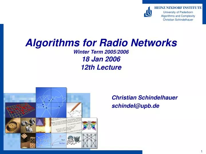
Algorithms for Radio Networks Winter Term 2005/2006 18 Jan 2006 12th Lecture. Christian Schindelhauer schindel@upb.de. Mobility in Wireless Networks (talk to be held at SOFSEM 2005). Introduction Wireless Networks in a Nutshelf Cellular Networks Mobile Ad Hoc Networks Sensor Networks

E N D
Algorithms for Radio NetworksWinter Term 2005/200618 Jan 200612th Lecture Christian Schindelhauer schindel@upb.de
Mobility in Wireless Networks(talk to be held at SOFSEM 2005) Introduction Wireless Networks in a Nutshelf Cellular Networks Mobile Ad Hoc Networks Sensor Networks Mobility Patterns Pedestrian Marine and Submarine Earth bound Vehicles Aerial Medium Based Outer Space Robot Motion Characterization of Mobility Patterns Measuring Mobility Patterns Models of Mobility Cellular Random Trip Group Particle based Combined Non-Recurrent Worst Case Discussion Mobility is Helpful Mobility Models and Reality
IntroductionThe history of Mobile Radio (I) • 1880s: Discovery of Radio Waves by Heinrich Hertz • 1900s: First radio communication on ocean vessels • 1910: Radios requried on all ocean vessels
IntroductionThe history of Mobile Radio (II) • 1914: Radiotelephony for railroads • 1918: Radio Transceiver even in war air plane • 1930s: Radio transceivers for pedestrians: “Walky-Talky” • 1940s: Handheld radio transceivers: “Handy-Talky”
IntroductionThe history of Mobile Radio (III) • 1970s Vint Cerfs Stanford Research Institute Van • First mobile packet radio tranceivers • ... • 2000s Wireless sensor coin sized sensor nodes Mica2dot from California based Crossbow company
Wireless Networks in a NutshelfCellular Networks • Static base stations • devide the field into cells • All radio communication is only • between base station and client • between base stations • usually hardwired • Mobility: • Movement into our out off a cell • Sometimes cell sizes vary dynamically (depending on the number of clients - UMTS) • Main problems: • Cellular Handoff • Location Service
Wireless Networks in a NutshelfMobile Ad Hoc Networks • MANET: • self-configuring network of mobile nodes • Nodes are routers and clients • no static infrastructure • network adapts to changes induced by movement • Positions of clients • in most applications not available • exceptions exist • Problems: • Find a multi-hop route between message source and target • Multicast a message • Uphold the network routing tables
Wireless Networks in a NutshelfWireless Sensor Networks • Sensor nodes • spacially distributed • equipped with sensors for • temperature, vibration, pressure, sound, motion, ... • Base stations • for collecting the information and control • possibly connected by ad-hoc-network • Main problem: • energy consumption • nodes are sleeping most of the time • read out the sensor information from the field
Mobility Patterns:Pedestrian • Characteristics: • Slow velocity • Dynamics from obstacles obstructing the signal • signal change a matter of meters • Applies for people or animals • Complete use of two-dimensional plane • Chaotic structure • Possible group behavior • Limited energy ressources • Examples • Pedestrians on the street or the mall • Wild life monitoring of animals • Radio devices for pets
Mobility Patterns:Marine and Submarine • Characteristics • Speed is limited due to friction • Two-dimensional motion • submarine: nearly three-dimensional • Usually no group mobility • except conoys, fleets, regattas, fish swarms • Reception • On the water: nearly optimal • Under the water: horrendous • solution: long frequencies or fsound
Mobility Patterns:Earth bound vehicles • Mobility by wheels • Cars, railways, bicycles, motor bikes etc. • Features • More speed than pedestrians • Nearly 1-dimensional mobility • because of collisions • Extreme group behavior • e.g. passengers in trains • Radio communication • Reflections of environment reduce the signal strengths dramatically • even of vehicles aiming at the same direction
Mobility Patterns:Aerial Mobility Examples: Flying patterns of migratory birds Air planes Characteristics High speeds Long distance travel problem: signal fading No group mobility except bird swarms Movement two-dimensional except air combat Application Collision avoidance Air traffic control Bird tracking
Mobility Patterns:Medium Based • Examples: • Dropwindsondes in tornadoes • Drifting buoyes • Chararcteristics of mobility • determined by the medium • can be often modelled by Navier-Stokes-equations • Medium can be 1,2,3-dimensional • Group mobility may occur • is unwanted, because no information • Location information is always available • this is the main purpose
Mobility Patterns:Outer Space • Characterization • Acceleration is the main restriction • Fuel is limited • Space vehicles drift through space most of the time • Non-circular orbits possible • Mobility in two-planet system is chaotic • Sometimes group behavior is desired, yet never been implemented • Radio communication • Perfect signal transmission • Energy resource usually no problem (solar paddles)
Mobility Patterns:Characterization • Group behavior • Can be exploited for radio communication • Limitations • Speed • Acceleration • Dimensions • 1, 11/2, 2, 21/2, 3 • Predictability • Simulation model • Completely erratic • Described by random process • Deterministic (selfish) behavior
Models of MobilityRandom Trip Mobility • Random Walk • Random Waypoint • Random Direction • Boundless Simulation Area • Gauss-Markov • Probabilistiic Version of the Random Walk Moblity • City Section Mobility Model
Models of Mobility:Group-Mobility Models • Exponential Correlated Random • Column Mobility • Nomadic Community Mobility • Pursue Mobility • Reference Point Group
Models of Mobility:Combined Mobility Models • Non-Recurrent Models
Models of Mobility:Worst-Cased Mobility Models • Pedestrian • Vehicular
ModelingWorst Case Mobility V: Pedestrian Model ↔ Maximum velocity ≤ vmax A: Vehicular Model ↔ Maximum accelaration ≤ amax
The Mobile Ad Hoc Network • As a start: synchronous round model In every round of duration Δ • Determine positions (speed vectors) of possible comm. partners • Establish (stable) communication links • Update routing information • Do the job, i.e. packet delivery, live video streams, telephone,…
The Mobility Model • Velocity bounded (pedestrian) mobility model for all i{1,…,n} • Acceleration bounded (vehicular) mobility model for all i{1,…,n} • Technical assumptions: • polynomial distances and speeds • complete knowledge of position
Crowds • Crowdedness of node set • natural lower bound on network parameters (like diversity) • Pedestrian (v) model: • Maximum number of nodes that can collide with a given node in time span [0,Δ] • Vehicular (a) model: • Maximum number of nodes that may move to node u meeting it with zero relative speed in time span [0,Δ] • crowd(S) := maxuS crowd(u)
Taming Mobility in the Link Layer • General Concept • Increase transmission distance • to guarrantee a certain life span Δ for each link • Apply the mobility model (i.e. amax or vmax is known) End position Transmission distance Start position
Transmission Range of Pedestrian Communication • Pedestrian model / Velocity bounded model • Sa-tisfiestriangleinequality Walking range end end start start
Transmission Range of Vehicular Communication start start end end • Vehicular mobility model / Acceleration bounded model • Sa-tisfiestriangleinequality
Mobile Radio Interferences An edge g interferes with edge e in the • Pedestrian (v) model • Vehicular (a) model p e q g No interference Interference e e e e p q g g g
Mobile Results (I) Theorem In both mobility models we observe for all connected graphs G: Lemma In both mobility models α{v,a}every mobile spanner is also a mobile power spanner, i.e. for some ß≥1 for all u,w S there exists a path (u=p0,p1,…,pk=w) in G such that:
Load, Congestion and Spanners • Interference number of the network G: • Int(G) := maxeE(G) |Int(e)| • Load and path system • Set of all message paths defines path system P • ℓ(e) := # number of packets sent over edge e according to P • Congestion of an edge (with respect to a path system P) • Congestion of a network G: • Mobile spanner • A network is a mobile spanner, if for all u,w exists a path (u=p0,p1,…,pk=w) such that for α{v,a}:
Mobile Results (II) Theorem Given a mobile spanner G for any of our mobility models then • for every path system P in a complete network C • there exists a path system P‘ in G such that Theorem The Hierarchical Grid Graph constitutes a mobile spanner with at most O(crowd(V) + log n) interferences (for both mobility models). The Hierarchical Grid Graph can be built up in O(crowd(V) + log n) parallel steps using radio communication
The Hierarchical Grid Graph(pedestrians) • Start with grid of box size Δ vmax • For O(log n) rounds do • Determine a cluster head per box • Build up star-connections from all nodes to their cluster heads • Erase all non cluster heads • Connect neighbored cluster heads • Increase box size by factor 2 • od
The Hierarchical Grid Graph(vehicular) t=2Δ t=0 t=Δ vx vx vx x x x • Algorithm: • Consider coordinates (x(si),y(si),x(s‘i),y(s‘i)) • Start with four-dimensional grid • with rectangular boxes of size (6Δ²amax, 6Δ²amax,2Δvmax,2Δvmax) • Use the same algorithm as before
Stable Basic Networks under Worst Case Mobility Corollary There exist distributed algorithms that construct a mobile network G for velocity bounded and acceleration bounded model with the following properties: • G allows routing approximating the optimal congestion by O(log² n) • Energy-optimal routing can be approximated by a factor of O(1) • G approximates the minimal interference number by O(log n) • The degree is O(crowd(S)+ log n) • The diameter is O(log n) • Still no routing can satisfy small congestion and energy at the same time!
Thanks for your attention!End of 12th lectureNext lecture: We 25 Jan 2006, 4pm, F1.110Next exercise class: Th 19 Jan 2006, 1.15 pm, F2.211 or Tu 24 Jan 2006, 1.15 pm, F1.110Next mini exam Mo 13 Feb 2006, 2pm, FU.511