Download
1 / 35
390 likes | 865 Views
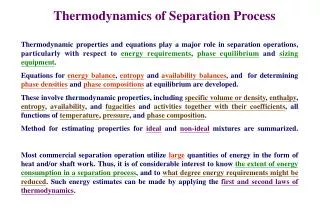
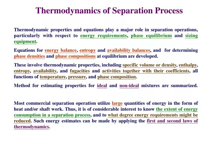
Thermodynamics of Separation Process. Thermodynamic properties and equations play a major role in separation operations, particularly with respect to energy requirements , phase equilibrium and sizing equipment .

E N D
Thermodynamics of Separation Process Thermodynamic properties and equations play a major role in separation operations, particularly with respect to energy requirements, phase equilibrium and sizing equipment. Equations for energy balance, entropy and availability balances, and for determining phase densities and phase compositions at equilibrium are developed. These involve thermodynamic properties, including specific volume or density, enthalpy, entropy, availability, and fugacities and activities together with their coefficients, all functions of temperature, pressure, and phase composition. Method for estimating properties foridealand non-ideal mixtures are summarized. Most commercial separation operation utilize large quantities of energy in the form of heat and/or shaft work. Thus, it is of considerable interest to know the extent of energy consumption in a separation process, and to what degree energy requirements might be reduced. Such energy estimates can be made by applying the first and second laws of thermodynamics.
Energy, Entropy and Availability Balances Consider the continuous, steady-state flow system for a general separation process in Figure 2.1. One or more feed streams flowing into the system are separated into two or more product streams that flow out of the system. Heat flows in or out of the system are denoted by Q, and shaft work crossing the boundary of the system is denoted by Ws. At steady state, if kinetic, potential, and surface energy changes are neglected, the first laws of thermodynamic (also referred to as the conservation of energy or the energy balance), states that the sum of all forms of energy flowing into the system equals the sum of the energy flows leaving the systems: n represents the molar flow rates zi represents the component mole fractions T represents the temperature P represents the pressure h represents the molar enthalpies s represents the molar entropies b represents the molar availability
All separation processes must satisfy the energy balance. Inefficient separation processes require large transfers of heat and/or shaft work both into and out of the process; efficient processes require smaller levels of heat transfer and/or shaft work. The first law of thermodynamics provides no information on energy efficiency, but the second law of thermodynamics (also referred to as the entropy balance) does. In words, the entropy balance is Unlike the energy balance, which states that energy is conserved, the entropy balance predicts the production of entropy, Sirr, which is the irreversible increase in the entropy of the universe. This sum, which must be a positive quantity, is a quantitative measure of the thermodynamic inefficiency of a process. In the limit, as a reversible process is approached, Sirr, tends to zero. Note that the entropy balance contains no terms related to shaft work.
Although Sirr is a measure of energy inefficiency, it is difficult to relate to this measure because it does not have the units of energy/time (power). A more useful measure or process inefficiency can be derived by combing Eqs. (*) and (**) to obtain a combined statement of the first and second laws of thermodynamics, which is given as This resulting equation is referred to as an availability (or exergy) balance, where the term availability means “available for complete conversion to shaft work.” The stream availability function, b, as defined by is a measure of the maximum amount of stream energy that can be converted into shaft work if the stream is taken to the reference state. It is similar to Gibbs free energy, g=h-Ts, but differs in that the infinite surrounding temperate, T0, appears in the equation instead of the stream temperature, T.
Terms in Eq (***) containing Q are multiplied by (1-T0/Ts), which, as shown in Figure 2.2, is the reversible Carnot heat-engine cycle efficiency, representing the maximum amount of shaft work that can be produced from Q at Ts, where the residual amount of energy (Q-Ws) is transferred as heat to sink at T0. Shaft work, Ws, remains at its full value in Eq (***). Thus, although Q and Ws have the same thermodynamic worth in Eq (*), heat transfer has less worth in Eq (***). This is because shaft wok can be converted completely to heat (by friction), but heat cannot be converted completely to shaft work unless the heat is available at an infinite temperature. Availability, like entropy, is not conserved in a real, irreversible process. The total availability (i.e., ability to produce shaft work) passing into a system is always greater than the total availability leaving a process. Thus Eq (***) is written with “into system” terms first. The difference is the lost work, LW, which is also called the loss of availability (or exergy), and is defined by Lost work is always a positive quantity. The greater its value, the greater is the energy inefficiency. In the lower limit, as a reversible process is approached, lost work tends to zero.
For any separation process, lost work can be computed from Eq (***). Its magnitude depends on the extent of process irreversibilities, which include fluid friction, heat transfer due to finite temperature-driving forces, mass transfer due to finite concentration or activity-driving forces, chemical reactions proceeding at finite displacements from chemical equilibrium, mixing of stream at differing conditions of temperature, pressure, and/or composition, and so on. Thus, to reduce lost work, driving force for momentum transfer, heat transfer, mass transfer, and chemical reaction must be reduce. Practical limits to this reduction exist because, as driving forces are decreased, equipment size increase, tending to infinitely large sizes as driving forces approach zero. For a separation process that occurs without chemical reaction, the summation of the stream availability functions leaving the process is usually greater than the same summation for streams entering the process. In the limit for a reversible process (LW=0), Eq (***) reduces to where Wmin is the minimum work required to conduct the separation and is equivalent to the difference in the heat transfer and shaft work terms in Eq (***). This minimum work is independent of the nature (or path) of the separation process. The work of separation for an actual irreversible process is always greater than the minimum value computed from Eq (****).
From Eq (***), it is seen that as a separation process becomes more irreversible and thus more energy inefficient, the increasing LW causes the required equivalent work of separation to increase by the same amount. Thus, the equivalent work of separation for an irreversible process is given by the sum of lost work and minimum work of separation. The second-law efficiency can be defined as
Example 2.1 For the propylene-propane separation of Figure 1.12, using the following thermodynamic properties for certain streams, as estimated from the Soave-Redlich-Kwong equation of state, and the relations given in Table 2.1, compute in SI units: (a) The condenser duty, QC (b) The reboiler duty, QR (c) The irreversible entropy production, assuming 303 K for the condenser cooling-water sink and 378 K for the reboiler steam source (d) The lost work, assuming T0=303 K (e) The minimum work of separation (f) The second-law efficiency
Phase Equilibrium Analysis of separation equipment frequently involves the assumption of phase equilibrium as expressed in terms of Gibbs free energy, chemical potentials, fugacities, activities. For each phase in a multiphase, multicomponent system, the total Gibbs free energy is where Ni=moles of species, i. At equilibrium, the total G for all phase is a minimum, and methods for determining this minimum are referred to as free-energy minimization techniques. Gibbs free energy is also the starting point for the derivation of commonly used equations for expressing phase equilibrium. From classical thermodynamics, the total differential of G is given by where i is the chemical potential or partial molar Gibbs free energy of species i. When the above equation is applied to a closed system consisting of two or more phases in equilibrium at uniform temperature and pressure, where each phase is an open system capable of mass transfer with another phase, then where the superscript (p) refers to each of N phases in equilibrium.
Conservation of moles of each species requires that which, upon substitution into Eq (*), gives With dNi(1) eliminated in Eq (**), each dNi(p) term can be varied independently of any other dNi(p) term. But this requires that each coefficient of dNi(p) in Eq (**) be zero. Therefore, Thus, the chemical potential of a particular species in a multicomponent system is identical in all phases at physical equilibrium.
Fugacities and Activity Coefficients At equilibrium,
K-Values An equilibrium ratio is the ratio of mole fractions of a species present in two phases at equilibrium. For the vapor-liquid case, the constant is referred to as the K-value or vapor-liquid equilibrium ratio: For the liquid-liquid case, the constant is referred to as the distribution coefficient or liquid-liquid equilibrium ratio: For the vapor-liquid case, relative volatility is defined by For the liquid-liquid case, relative selectivity is defined by
Example 2.2 Estimate the K-values of a vapor-liquid mixture of water and methane at 2 atm total pressure for temperatures of 20 and 80 C.
Ideal Gas, Ideal Liquid Solution Model Design procedures for separation equipment require numerical values for phase enthalpies, entropies, densities, and phase equilibrium ratios. Classical thermodynamics provides a means for obtaining these quantities in a consistent manner from P-v-T relationships, which are usually referred to as equation-of-state models. The simplest model applies when both liquid and vapors are ideal solutions (all activity coefficients equal 1.0) and the vapor is an ideal gas. The thermodynamic properties can be computed from unary constants for each of the species in the mixture in a relatively straightforward manner using the equations given in Table 2.4. In general, these equations apply only at near-ambient pressure, up to about 50 psia (345 kPa), for mixtures of isomers or components of similar molecular structure.
A common empirical representation of the effect of temperature on the zero-pressure vapor heat capacity, Cp0V, of a pure composition is the following third-degree polynomial equation: The ideal gas species molar enthalpy is The ideal gas species molar entropy is The vapor pressure of a pure liquid species is well represented over a wide range of temperature from below the normal boiling to the critical region by an empirical extended Antoine equation: At low pressures, the enthalpy of vaporization is given in terms of vapor pressure by classical thermodynamics:
Example 2.3 Styrene is manufactured by catalytic dehydrogenation of ethylbenzene, followed by vacuum distillation to separate styrene from unreacted ethylbenzene. Typical conditions for feed to a commercial distillation unit are 77.5 C (350.65 K) and 100 torr (13.332 kPa) with the following vapor and liquid flows at equilibrium: Based on the property constants given left, and assuming that the ideal gas, ideal liquid solution model of Table 2.4 is suitable at this low pressure, estimate values of vV, V, hV, sV, vL, L, hL, sL, in SI units, and the K-values and relative volatility.
Graphical Correlations of Thermodynamic Properties Saturated liquid densities as a function of temperature are plotted for some hydrocarbons in Figure 2.3. The density decreases rapidly as the critical temperature is approached until it becomes equal to the density of the vapor phase at the critical point. The liquid density curves are well correlated by the modified Rachett equation.
Figure 2.4 is a plot of liquid-state vapor pressures of some common chemicals, covering a wide range of temperature from below the normal boiling point to the critical temperature, where the vapor pressure terminates at the critical pressure. In general, the curves are found to fit the extended Antoine equation reasonably well. This plot is particularly useful for determining the phase state (liquid or vapor) of a pure substance and for computing Raoult’s law K-values.
Curves of ideal gas, zero-pressure enthalpy over a wide range of temperature are given in Figure 2.5 for light paraffin hydrocarbon. The datum is the liquid phase at 0 C, at which the enthalpy is zero. The derivates of these curves fit the third-degree polynomial for the ideal gas heat capacity reasonably well. Curves of ideal-gas entropy of several light gases, over a wide range of temperature, are given in Figure 2.6.
Enthalpies (heats) of vaporization are plotted as a function of saturation temperature in Figure 2.7 for light paraffin hydrocarbons. These values are independent of pressure and decrease to zero at the critical point, where vapor and liquid phases become indistinguishable. These plots, together with the ideal-gas enthalpy of Figure 2.5, can be used with Eq. (5) of Table 2.4 to compute liquid enthalpy up to temperatures corresponding to a vapor pressure of about 350 kPa.
Nomographs for estimating K-values of hydrocarbons and light gases are presented in Figure 2.8 and 2.9, which are taken from Hadden and Grayson. In both charts all K-values collapse to 1.0 at a pressure of 5,000 psia (34.5 MPa). This pressure, called the convergence pressure, depends on the boiling range of the components in the mixture. For example, in Figure 2.10 the components of mixture (N2 to nC10) cover a very wide boiling-point range, resulting in convergence pressure of close to 2,500 psia. For narrow-boiling mixtures, such as a mixture of ethane and propane, the convergence pressure is generally less than 1,000 psia. The K-value charts of Figures 2.8 and 2.9 apply strictly to a convergence pressure of 5,000 psia, but can be used without correlation to make preliminary estimates.
Example 2.4 Petroleum refining begins with the distillation, at near-atmospheric pressure, of crude oil into fractions of different boiling ranges. The fraction boiling from 0 to 100 C, the light naphtha, is a blending stock of gasoline. The fraction boiling from 100 to 200 C, the heavy naphtha, undergoes subsequent chemical processing into more useful products. One such process is steam cracking to produce a gas containing ethylene, propylene, and a number of other compounds, including benzene and toluene. This gas is then sent to a distillation train to separate the mixture into a dozen or more products. In the first column, hydrogen and methane are removed by cryogenic distillation at 3.2 MPa (464 psia). At a tray in the distillation column where the temperature is 40 F, use the appropriate K-value nomography to estimate K-values for H2, CH4, C2H4, and C3H6.
Nonideal Thermodynamic Property Models Unlike the equations of Table 2.1, which are universally applicable to all pure substances and mixtures, where ideal or nonideal, nouniversal equations are available for computing, for nonideal mixtures, values of thermodynamic properties such as density, enthalpy, entropy, fugacities, and activity coefficients as functions of temperature, pressure, and phase composition. Instead, two types of models are used: (1) P-v-T equation-of-state models (2) activity coefficient or free-energy models These are based on constitutive equations because they depend on the constitution or nature of the components in the mixture.
P-v-T Equation-of-state Models -a relationship between molar volume (or density), temperature, and pressure A large number of such equations has been proposed, mostly for the vapor phase. The simplest is the ideal gas law, which applies only at low pressures or high temperatures because it neglects the volume occupied by the molecules and intermolecular forces among the molecules. All other equations of state attempt to correct for these two deficiencies. The equations of state that are most widely used by chemical engineers are listed in Table 2.5.
Not included in Table 2.5 is the van der Waals equation, P=RT/(v-b)-a/v2, where a and b are species-dependent constants that can be estimated from the critical temperature and pressure. The van der Waals equation was the first successful approach to the formulation of an equation of state for a nonideal gas. It is rarely used by chemical engineers because its range of application is too narrow. However, its development did suggest that all species might have equal reduced molar volumes, vr=v/vc, at the same reduced temperature, Tr=T/Tc, and reduced pressure, Pr=P/Pc. This finding, referred to as the law of corresponding states, was utilized to develop the generalized equation of sate given as Eq. (2) in Table 2.5. That equation defines the compressibility factor, Z, which is a function of Pr, Tr, and the critical compressibility, Zc, or the acentric factor, , which is determined from experimental P-v-T data. The acentric factor, introduced by Pitzer et al., accounts for differences in molecular shape and is determined from the vapor pressure curve: This definition results in value for of zero for symmetric molecules. Some typical values of are 0, 0.263, 0.489, and 0.644 for methane, toluene, n-decane, and ethyl alcohol, respectively, as taken from the extensive tabulation of Reid et al..
Equation (*), which is cubic in Z, can be solved analytically for three roots (e.g., see Perry’s Handbook, 6th ed., pp. 2-15). In general, at supercritical temperature, where only one phase can exist, one real root and a complex conjugate pair of roots are obtained. Below the critical temperature, where vapor and/or liquid phases can exist, three real roots are obtained, with the largest value of Z (largest v) corresponding to the vapor phase-that is, Zv-and the smallest Z (smallest v) corresponding to the liquid phase-that is, ZL. The intermediate value of Z is of no practical use. To apply the R-K equation to mixtures, mixing rules are used to average the constants a and b for each component in the mixture. The recommended rules for vapor mixtures of C components are
Example 2.5 Glanville, Sage, and Lacey measured specific volume of vapor and liquid mixtures of propane and benzene over wide ranges of temperature and pressure. Use the R-K equation to estimate specific volume of a vapor mixture containing 26.92 wt% propane at 400 F (477.6 K) and a saturation pressure of 410.3 psia (2,829 kPa). Compare the estimated and experimental values.
R-K-S equation of state was immediately accepted for application to mixtures containing hydrocarbons and/or light gases because of its simplicity and accuracy. The main improvement was to make the parameter a a function of the acentric factorand temperature so as to achieve a good fit to vapor pressure data of hydrocarbons and thereby greatly improve the ability of the equation to predict properties of the liquid phase. Peng and Robinson presented a further modification of the R-K and S-R-K equations in an attempt to achieve improved agreement with experimental data in the critical region and for liquid molar volume. The S-R-K and P-R equations of state are widely applied in process calculations, particularly for saturated vapors and liquids. When applied to mixtures of hydrocarbons and/or light gases, the mixing rules are given by Values of kij, back-calculated from experimental data, have been published for both the S-R-K and P-R equations. Generally, kij is taken as zero for hydrocarbons paired with hydrogen or other hydrocarbons. Although the S-R-K and P-R equations were not intended to be applied to mixtures containing polar organic compounds, they are finding increasing use in such applications by employing large values of kij, in the vicinity of 0.5, as back- calculated from experimental data.
Derived Thermodynamic Properties from P-v-T Models ideal gas law R-K equation
The fugacity coefficient, , of a pure species at temperature T and pressure P from the R-K equation applies to the vapor for P<Ps. For P>Ps, is the fugacity coefficient of the liquid. Saturation pressure corresponds to the condition of v=L. Thus, at a temperature T<Tc, the saturation pressure (vapor pressure), Ps, can be estimated from the R-K equation of state by setting Eq. (*) for the vapor equal to Eq. (*) for the liquid and solving for P, which then equals Ps, by an iterative procedure. These results are plotted in reduced form in Figure 2.12. The R-K vapor pressure curve does not satisfactorily represent data for a wide range of molecular shapes, as witnessed by the experimental curves for methane, toluene, n-decane, and ethyl alcohol on the same plot. This failure represents one of the major shortcomings of the R-K equation and is the main reason why Soave modified the R-K equation by introducing the acentric factor in such a way as to greatly improve agreement with experimental vapor pressure data. Thus, while the critical constants, Tc and Pc alone are insufficient to generalize thermodynamic behavior, a substantial improvement is made by incorporating into the P-v-T equation a third parameter that represents the generic differences in the reduced vapor pressure curves.
Ideal K-values as determined from Eq.(7) in Table 2.4, depend only on temperature and pressure, and not on composition. Most frequently, ideal K-values are applied to mixtures of nonpolar compounds, particularly hydrocarbons such paraffins and olefins. Figure 2.13 shows experimental K-value curves for a light hydrocarbon, ethane, in various binary mixtures with other, less volatile hydrocarbons at 100 F (310.93 K) for pressure from 100 psia (689.5 kPa) to convergence pressures between 720 and 780 psia (4.964 MPa to 5.378 MPa). At the convergence pressure, separation by operations involving vapor-liquid equilibrium becomes impossible because all K-values become 1.0. Figure 2.13 shows that ethane does not form ideal solutions at 100 F with all the other components because the K-values depend on the other components. For example, at 300 psia, the K-value of ethane in benzene is 80% higher than in propane.
Example 2.6 In the high-pressure, high-temperature thermal hydrodealkylation of toluene to benzene (C7H8+H2C6H6+CH4), excess hydrogen is used to minimize cracking of aromatics to light gases. In practice, conversion of toluene per pass through the reactor is only 70%. To separate and recycle hydrogen, hot reactor effluent vapor of 5,597 kmol/h at 500 psia (3,448 kPa) and 275 F (408.2 K) is partially condensed to 120 F (322 K), with product phases separated in a flash drum. If the composition of the reactor effluent is as follows, and the flash drum pressure is 485 psia (3,444 kPa), calculate equilibrium compositions and flow rates of vapor and liquid leaving the flash drum and the amount of heat that must be transferred using a computer-aided, steady-state simulation program with each of the equation-of-state models discussed above. Compare the results, including flash drum K-values and enthalpy and entropy changes.
Solution Because the reactor effluent is mostly hydrogen and methane, the effluent at 275 F and 500 psia, and the equilibrium vapor at 120 F and 485 psia are nearly ideal gas (0.98<Z<1.00), despite the moderately high pressure. Thus, the enthalpy and entropy changes are dominated by vapor heat capacity and latent heat effects, which are largely independent of which equation of state is used. Consequently, the enthalpy and entropy changes among the three equations of state differ by less than 2%. Significant differences exist for the K-values of H2 and CH4. However, because the values are in all cases large, the effect on the amount of equilibrium vapor is very small. Reasonable K-values for H2 and CH4, based on experimental data, are 100 and 13, respectively. K-values for benzene and toluene differ among the three equations of state by as much as 11% and 14%, respectively, which, however, causes less than a 2% difference in the percentage of benzene and toluene condensed. Raoult’s law K-values for benzene and toluene, based on vapor pressure data, are 0.01032 and 0.00350, which are considerably lower than the values computed from each of the three equations of state because deviations to fugacities due to pressure are important in the liquid phase and, particularly, in the vapor phase.