Download
1 / 40
501 likes | 731 Views
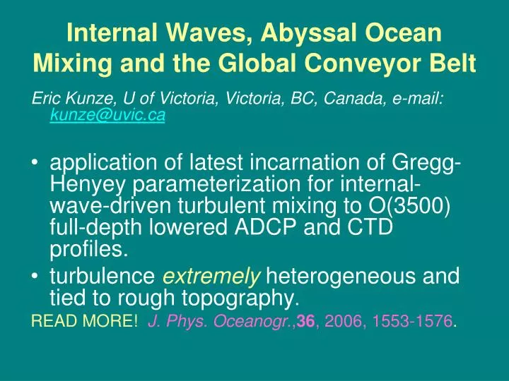
Internal Waves, Abyssal Ocean Mixing and the Global Conveyor Belt. Eric Kunze, U of Victoria, Victoria, BC, Canada, e-mail: kunze@uvic.ca

E N D
Internal Waves, Abyssal Ocean Mixing and the Global Conveyor Belt Eric Kunze, U of Victoria, Victoria, BC, Canada, e-mail: kunze@uvic.ca • application of latest incarnation of Gregg-Henyey parameterization for internal-wave-driven turbulent mixing to O(3500) full-depth lowered ADCP and CTD profiles. • turbulence extremely heterogeneous and tied to rough topography. READ MORE!J. Phys. Oceanogr.,36, 2006, 1553-1576.
Why Abyssal Mixing? • cold dense water formed at high latitudes fills the abyssal ocean. • What is the return path for the bottom water? • Munk (1966) Munk and Wunsch (1998) claim mixing with overlying waters needed to close thermohaline circulation below 1-km depth.
Historical Sidenote • during Permian, Earth was tropical and temperate → no cold-water formation. • bottom-water ventilation to abyss shut down. • over several thousand years, abyssal waters warmed to surface temperatures of 16ºC and abyssal O2 used up and abyss became anoxiclike the Black Sea. • has been speculated that overturning release of CO2 and sulfide gases caused the Permian mass extinction.
Abyssal Mixing • Munk (1966) argued basin-average diffusivity of eddy diffusivity 10–4 m2/s. • mixing could be interior (A), where isopycnals outcrop at high latitudes (B), or impinge rough topography (C). • observations rule out (A) • mixing elevated for (C) but not enough (Kunze and Toole 1997 JPO).
Internal-Wave-Generated Turbulence • in most of stratified ocean interior, turbulence is driven by internal wave breaking. • wave/wave interaction theory (McComas and Müller 1981; Henyey et al. 1986) predicts rate of energy transfer to smallscale and turbulence. • verified to within a factor of 2 (Gregg 1989; Polzin et al. 1995; Gregg et al. 2003) K = O(10–5 m2/s) in most ocean. • falls short in canyons, on continental shelves and in internal-wave generation regions.
Gregg et al. (Nature 2003) eddy diffusivity depends on • shear variance • strain variance (thru shear/strain ratio Rω) •f/N (K→ 0 as f/N→ 0) ●K0 = 0.05 × 10⁻⁴ m2/s Parameterization
Data Analysis • lowered ADCP/CTD profiles of 10-20 m velocity u, v, and 1-2 m temperature T and salinity S. • broken into half-overlapping 350-m segments starting at the bottom 40k segments. • strain ξzfrom (N2 – <N2>)/<N2> where background stratification <N2> based on a quadratic fit over segment (contaminated by sharp pycnoclines at low latitudes and thermohaline intrusioins). • each segment windowed and Fourier-transformed.
Vertical Wavenumber Spectra Strain spectra (solid): • saturated at high wavenumber. • excess redness at lowest wavenumbers. Shear spectra (thick dot): • affected by instrument noise (thin dots) for wavelengths < 150 m.
Shear/Strain Ratio Rω vs. N for N > 5 ×10⁻⁴ rad/s, shear/strain ratio is 7 (GM = 3). for N < 5 ×10⁻⁴ rad/s, instrument noise dominates shear. instrument noise
Summary 1: Internal Waves • strain spectra saturated at high wavenumber with kcE ~ constant. • shear spectra strongly influenced by instrument noise which overwhelms any signal for N < 5 × 10⁻⁴ rad/s. • shear/strain ratio Rω =7, implying a stronger near-inertial peak than in GM model.
Egbert and Ray Surface Tide Loss • higher vertically-integrated dissipation rates associated with rough topography. • sites of surface tide loss. • note that most (90%) surface tide ‘dissipation’ radiates away as low-mode internal tides.
Indian Ocean (10ºN) barotropic and 500-mab velocity vertically-integrated dissipation rate ε topographic roughness var(H) inertial winds and tidal currents diffusivity K (white GM 10−5 m2/s, bluelower, red higher)
Summary 2: Dissipation Rates • vertically-integrated dissipation rates ∫ε mostly comparable to GM-expected values O(1 mW/m2). • higher dissipations found over rough topography, occasionally slightly exceeding (by a factor of 3) average deep-ocean tidal dissipations. • where do tides dissipate?
Average Profiles • as functions of depth z, height h, neutral density γn, buoyancy frequency N. • K ~ 0.1 × 10⁻⁴ m2/s in upper 3 km, increasing to 0.3-0.4 toward bottom. • strain-based K a factor of 2-3 larger in upper ocean due to contamination by pycnoclines and intrusions. • inverse estimates of K ~ O(10–4 m2/s) in abyss (hydraulic flow through passages?).
Latitude-Depth Dependence • K increases with depth in tropics and subtropics. • above 3000-m depth, K increases with latitude. • in abyss, max K of O(10−4 m2/s) at 20-30º. • maximum diapycnal w* 0.5 cm/day at 40-60º and 4000-m depth but evidence for 2 upwelling cells.
Summary 3: Diapycnal Velocities • diapycnal velocities w* upward everywhere, strongest at high latitudes below 3500 and above 2000 m (0.3-0.5 cm/day) with weak or vanishing w* in intermediate depths.
Bottom Diffusivity Kb • depends both on bottom roughness var(H) [to 1/4] and semidiurnal surface tidal velocity Vsemi[to 1/8].
Summary 4: Diffusivity • for most of ocean, inferred diffusivity <K> is O(0.1 × 10⁻⁴ m2/s). • much weaker within 10º of equator because of j(f/N). • approaches 10−4 m2/s in high-latitude 500-1000 mab. • high K extends into pycnocline over rough topography in conjunction with strong tidal currents and Antarctic Circumpolar Current (AACC). • strain-based K with R= 7 overestimatesby factor of 2 in upper ocean (sharp pycnoclines, thermohaline intrusions?) and underestimates by factor of 4 in Southern Ocean (possibly shear noise?).
Why Weak Mixing? • thermohaline circulation more complicated than 1-D Munk model with Deep and Intermediate Waters intervening between Bottom Water and pycnocline. • Bottom Water need only mix with overlying Deep Water which outcrops at high latitudes to be transformed into Bottom and Intermediate Waters.
Implications • return path of Bottom Water NOTuniform upwelling but intensified localized hotspots over rough topography. • abyssal mixing is stronger, perhaps strong enough since Bottom Water need only mix with the overlying Deep Water. • stratification of waters above 3000 m controlled by interleaving Deep and Intermediate Waters, NOT mixing. • deep-ocean tidal dissipation unaccounted for but abrupt topography and near-critical continental slopes undersampled. • strain-based diffusivities in right ballpark.
Caveats • parameterization only includes internal-wave-driven turbulence, excluding hydraulically-controlled flow through passages and direct turbulence production near bottom. It does not work everywhere. • shear measurements very noisy. • spectral estimation method coarse in the vertical (350 m) Cthulhu fthagn Rlyeh
Biologically-Generated Turbulence during 28 APR 2005 dusk migration of the backscatter layer in Saanich Inlet, turbulent dissipation rates were 1000 higher than normal for 15 minutes. supported theoretical estimates Huntley and Zhou (2005) and Dewar et al. (2006) that biological mixing could be as important as tides and wind. READ MORE Science 2006
On Further Work • Shani Rousseau collected 11 more dusk/dawn time-series in Saanich Inlet and 6 at Ocean Station Papa for her Masters research with no recurrence of burst (submitted to JPO). • so APR 2005 burst a rare event and biologically-generated mixing not important in the ocean.
Indian Ocean (32ºS) vertically-integrated dissipation rate ε topographic roughness var(H) inertial winds and tidal currents diffusivity K (white GM 10−5 m2/s, bluelower, red higher)