Download

1 / 36
380 likes | 421 Views
On the Environmental Kuznets Curve: A Real Options Approach . Masaaki Kijima, Katsumasa Nishide and Atsuyuki Ohyama Tokyo Metropolitan University Yokohama National University NLI Research Institute. Introduction Optimal Environmental Policy Why Does the Kuznets Curve Present ? Conclusions.

E N D
On the Environmental Kuznets Curve: A Real Options Approach Masaaki Kijima,Katsumasa Nishide andAtsuyuki Ohyama Tokyo Metropolitan University Yokohama National University NLI Research Institute
Introduction Optimal Environmental Policy Why Does the Kuznets Curve Present ? Conclusions • Model setup : A real options approach • Thresholds for stopping and restarting • Model setup : Alternating renewal processes • Transition density of the pollution level • The inverse-U-shaped pattern as expected pollution level • Numerical example
What is the Kuznets Curve ? • The Kuznets Curve reveals that Income differential first increases due to the economic growth; but then starts decreasing to settle down • Kuznets (1955,1973);Robinson (1976); Barro (1991); Deininger and Squire (1996); Moran (2005), etc.
Literature Review • Environmental Kuznets Curve Similar curves are observed in various pollution levels 【Empirical studies】 • Grossman and Krueger (1995) • Shafik and Bandyopadhyay (1992) • Panayotou (1993) Many other empirical studies, while just a few theoretical research 【Theoretical studies】 • Lopez (1994) • Selden and Song (1995) • Andreoni and Levinson (2001)
Itaru Yasui, "Environmental Transition - A Concept to Show the Next Step of Development“ .Symposium on Sustainability in Norway and Japan: Two Perspectives. April 26, 2007 NTNU, Trondheim, Norway
Lopez (1994) • Macroeconomic model (no uncertainty) • - the production is affacted by the level of pollution • - in the optimal path, pollution is U-shaped w.r.t. the production. • Selden and Song (1995) • Representative agent in a dynamic setting (no uncertainty) • - utility from consumption and disutility from pollution • if the abatement function satisfies some property, the agent switches the strategy when the pollution touches a certain level.
Andreoni and Levinson (2001) Representative agent in a static setting (no uncertainty) - utility from consumption and disutility from pollution - if the elasticity of pollution w.r.t. the abatement effort is large enough, the agent pays a more amount of abatement cost as his income becomes larger. In the previous literature, ・ uncertainty is not considered, ・ macroeconomic effect is not examined as the aggregation of microeconomic behavior.
Purpose • Our purpose is to present a simple model to explain the inverse-U-shaped pattern using a real options model. What is the optimal management of stock pollutants? Derive the thresholds of regulation and de-regulation. As a result,… • How will stock pollutants change in time? • How about expected stock pollutants in total ? An inverse-U-shaped pattern (=Environmental Kuznets Curve) Micro’s perspective A real options approach Alternating renewal processes Macro’s perspective
Two Ingredients • Real Options Approach (strategic) switching model under uncertainty • Dixit and Pindyck (1997), etc. We use the same framework as Dixit and Pindyck (1994, Chapter 7) and Wirl (2006) • Alternating renewal processes Switchings produce ‘on’ and ‘off’ alternately with iid lifetimes – Ross (1996), etc.
Model Setup: A Real Options Approach • From the micro’s perspective, we analyze each country i • Stock Pollutants : where k represents each regime as shown below. • Cost of external Effects: • Benefit in regime k : • Government chooses alternative regimes for an environmental policy: one under regulations L and the other under de-regulations H (including no regulation). Of course, it is possible to switch the regimes.
The country i’s problem • Under the de-regulation regime, the value function is • Under the regulation regime, the value function is where A is a constant, where B is a constant,
Thresholds for Stopping and Restarting • We derive two thresholds: one for starting regulation , and the other for de-regulation . These equations have four unknowns; i.e. the two thresholds , , and the coefficients and . Therefore, we can obtain the solution at least numerically. Smooth-pasting Condition Value-matching Condition
Model Setup: Alternating Renewal Process We calculate the transition density of the pollution level using the theory of alternating renewal processes, and then, illustrate the inverse-U-shaped pattern. 【Assumption】 Instead of , we investigate the shape of. Therefore, we consider the following stochastic process. Suppose that countries execute optimally the switching options for regulating and de-regulating pollutions in time.
<<Alternating Renewal Process>> Consider a system that can be in one of two states: on (regulation) or off (de-regulation). Regulation De-regulation off on off off on on on off off • Let , be the sequences of durations to switch the states. The sequences , are independent and identically distributed (iid) except . • Suppose that , . 【Thresholds】
The transition probability density for country i: To simplify our notation, we omit the superscript i for a while. 【Definition of the hitting times】 with and also
Duration Density Function Sinceandare independent, we denote Also, we denote whereis the convolution operator. The sequenceis called a (delayed) alternating renewal process.
【Delayed renewal processes】 【Renewal functions】 <<Renewal densities>> By the definition,
Also, following the basic renewal theory, we obtain Laplace Transform Laplace Transform Inverse Laplace Transform Inverse Laplace Transform via numerical inversion
Renewal Functions: , In this case, after Time=300, then Time State Equal Time Time
Transition Probability of the Pollution Level 【Notation】 In order to calculate , we define and denote These transition densities are known in closed form for the case of geometric Brownian motions. Also, we denote the regime at time t by . Note that, because , we have
【To calculate the transition probability density, we consider the following three cases】 Case 1: , that is, Case 2: and that is, Case 3: and that is, These 3 cases are mutually exclusive and exhaust all the events.
【Case 1】 【Case 2】 In this case, the event to hit at some time s has occurred.
【Case 3】 Transition density is given by State Density Time
From the basic renewal theory, as , we have Hence, when and , we obtain
The Inverse-U-Shaped Pattern 【A Model for the Aggregated Level】 Consider the sum of each country’s log-stock pollutant where with subject to the switching at
【Assumptions】 Because each country’s economic scale is different, its initial stock pollutant is distinct over countries. The uncertainties (Brownian motions) are mutually independent, because each country executes environmental policy non-cooperatively. Because environmental problems are the world-wide issue, technological transfers are smoothly performed; so that it is plausible to assume the parameters to be the same over countries, i.e. The switching thresholds are the same over the countries.
Under these assumptions, is a weighted average of independent replicas with different initial states. • Hence, in principle, we can calculate the transition probability density of • However, when N is sufficiently large, the effect from the law of large numbers (or the central limit theorem) becomes dominant, and we are interested in the mean (or the variance) of . That is, • Moreover, as the first approximation, we consider
Numerical Examples We are interested in the shape of with respect to t with
The Environmental Kuznets Curve • An inverse-U-shaped pattern GDP per capita also grows in average exponentially in time.
We describe a simple real options (switching) model to explain why the environmental Kuznets curve presents for various pollutants when each country executes its environmental policy optimally. • The transition probability density of the pollution level is derived using the alternating renewal theory. • In particular, its mean is calculated numerically to show the inverse-U-shaped pattern. • The assumption of GBM can be removed as far as the constant switching thresholds and the Laplace transform of the first hitting time to the thresholds are known. • As a future work, our model can be applied to estimate when the peak of the curve will present.