Download
1 / 67
670 likes | 779 Views
Image Formation. CSc I6716 Fall 2010. Topic 1 of Part I Image Formation. Zhigang Zhu, City College of New York zhu@cs.ccny.cuny.edu. Acknowledgements. The slides in this lecture were kindly provided by Professor Allen Hanson University of Massachusetts at Amherst. Lecture Outline.

E N D
Image Formation CSc I6716 Fall 2010 Topic 1 of Part I Image Formation Zhigang Zhu, City College of New York zhu@cs.ccny.cuny.edu
Acknowledgements The slides in this lecture were kindly provided by Professor Allen Hanson University of Massachusetts at Amherst
Lecture Outline • Image Formation Basic Steps • Geometry • Pinhole camera model & Thin lens model • Perspective projection & Fundamental equation • Radiometry • Photometry • Color, human vision, & digital imaging • Digitalization • Sampling, quantization & tessellations • More on Digital Images • Neighbors, connectedness & distances
Lecture Outline • Image Formation Basic Steps • Geometry • Pinhole camera model & Thin lens model • Perspective projection & Fundamental equation • Radiometry • Photometry • Color, human vision, & digital imaging • Digitalization • Sampling, quantization & tessellations • More on Digital Images • Neighbors, connectedness & distances
Abstract Image • An image can be represented by an image function whose general form is f(x,y). • f(x,y) is a vector-valued function whose arguments represent a pixel location. • The value of f(x,y) can have different interpretations in different kinds of images. Examples Intensity Image - f(x,y) = intensity of the scene Range Image - f(x,y) = depth of the scene from imaging system Color Image - f(x,y) = {fr(x,y), fg(x,y), fb(x,y)} Video - f(x,y,t) = temporal image sequence
Basic Radiometry • Radiometry is the part of image formation concerned with the relation among the amounts of light energy emitted from light sources, reflected from surfaces, and registered by sensors.
Light and Matter • The interaction between light and matter can take many forms: • Reflection • Refraction • Diffraction • Absorption • Scattering
Lecture Assumptions • Typical imaging scenario: • visible light • ideal lenses • standard sensor (e.g. TV camera) • opaque objects • Goal To create 'digital' images which can be processed to recover some of the characteristics of the 3D world which was imaged.
Steps World Optics Sensor Signal Digitizer Digital Representation World reality Optics focus {light} from world on sensor Sensor converts {light} to {electrical energy} Signal representation of incident light as continuous electrical energy Digitizer converts continuous signal to discrete signal Digital Rep. final representation of reality in computer memory
Factors in Image Formation • Geometry • concerned with the relationship between points in the three-dimensional world and their images • Radiometry • concerned with the relationship between the amount of light radiating from a surface and the amount incident at its image • Photometry • concerned with ways of measuring the intensity of light • Digitization • concerned with ways of converting continuous signals (in both space and time) to digital approximations
Lecture Outline • Image Formation Basic Steps • Geometry • Pinhole camera model & Thin lens model • Perspective projection & Fundamental equation • Radiometry • Photometry • Color, human vision, & digital imaging • Digitalization • Sampling, quantization & tessellations • More on Digital Images • Neighbors, connectedness & distances
Geometry • Geometry describes the projection of: three-dimensional (3D) world two-dimensional (2D) image plane. • Typical Assumptions • Light travels in a straight line • Optical Axis: the axis perpendicular to the image plane and passing through the pinhole (also called the central projection ray) • Each point in the image corresponds to a particular direction defined by a ray from that point through the pinhole. • Various kinds of projections: • - perspective - oblique • - orthographic - isometric • - spherical
Basic Optics • Two models are commonly used: • Pin-hole camera • Optical system composed of lenses • Pin-hole is the basis for most graphics and vision • Derived from physical construction of early cameras • Mathematics is very straightforward • Thin lens model is first of the lens models • Mathematical model for a physical lens • Lens gathers light over area and focuses on image plane.
Pinhole Camera Model • World projected to 2D Image • Image inverted • Size reduced • Image is dim • No direct depth information • f called the focal length of the lens • Known as perspective projection
Pinhole camera image Amsterdam Photo by Robert Kosara, robert@kosara.net http://www.kosara.net/gallery/pinholeamsterdam/pic01.html
Equivalent Geometry • Consider case with object on the optical axis: • More convenient with upright image: • Equivalent mathematically
f o i OPTIC AXIS 1 1 1 f i o IMAGE PLANE ‘THIN LENS LAW’ = + LENS Thin Lens Model • Rays entering parallel on one side converge at focal point. • Rays diverging from the focal point become parallel.
Coordinate System • Simplified Case: • Origin of world and image coordinate systems coincide • Y-axis aligned with y-axis • X-axis aligned with x-axis • Z-axis along the central projection ray
Perspective Projection • Compute the image coordinates of p in terms of the world coordinates of P. • Look at projections in x-z and y-z planes
x X = f Z+f fX x = Z+f X-Z Projection • By similar triangles:
y Y = f Z+f fY y = Z+f Y-Z Projection • By similar triangles:
fY fX y x = = Z+f Z+f Perspective Equations • Given point P(X,Y,Z) in the 3D world • The two equations: • transform world coordinates (X,Y,Z) into image coordinates (x,y) • Question: • What is the equation if we select the origin of both coordinate systems at the nodal point?
Reverse Projection • Given a center of projection and image coordinates of a point, it is not possible to recover the 3D depth of the point from a single image. In general, at least two images of the same point taken from two different locations are required to recover depth.
P(X,Y,Z) Stereo Geometry • Depth obtained by triangulation • Correspondence problem: pl and pr must correspond to the left and right projections of P, respectively.
Lecture Outline • Image Formation Basic Steps • Geometry • Pinhole camera model & Thin lens model • Perspective projection & Fundamental equation • Radiometry • Photometry • Color, human vision, & digital imaging • Digitalization • Sampling, quantization & tessellations • More on Digital Images • Neighbors, connectedness & distances
Radiometry • Image: two-dimensional array of 'brightness' values. • Geometry: where in an image a point will project. • Radiometry: what the brightness of the point will be. • Brightness: informal notion used to describe both scene and image brightness. • Image brightness: related to energy flux incident on the image plane: => IRRADIANCE • Scene brightness: brightness related to energy flux emitted (radiated) from a surface: => RADIANCE
Radiometry & Geometry • Goal: Relate the radiance of a surface to the irradiance in the image plane of a simple optical system.
2 p d E = 4 cos a i -f 4 L s Radiometry Final Result • Image irradiance is proportional to: • Scene radiance Ls • Focal length of lens f • Diameter of lens d • f/d is often called the f-number of the lens • Off-axis angle a
Cos a Light Falloff 4 Lens Center Top view shaded by height y x -p/2 p/2 -p/2
Lecture Outline • Image Formation Basic Steps • Geometry • Pinhole camera model & Thin lens model • Perspective projection & Fundamental equation • Radiometry • Photometry • Color, human vision, & digital imaging • Digitalization • Sampling, quantization & tessellations • More on Digital Images • Neighbors, connectedness & distances
Photometry • Photometry: Concerned with mechanisms for converting light energy into electrical energy. World Optics Sensor Signal Digitizer Digital Representation
Color Representation B • Color Cube and Color Wheel • For color spaces, please read • Color Cube http://www.morecrayons.com/palettes/webSmart/ • Color Wheel http://r0k.us/graphics/SIHwheel.html • http://www-viz.tamu.edu/faculty/parke/ends489f00/notes/sec1_4.html H I S G R
Digital Color Cameras • Three CCD-chips cameras • R, G, B separately, AND digital signals instead analog video • One CCD Cameras • Bayer color filter array • http://www.siliconimaging.com/RGB%20Bayer.htm
Human Eyes & Color Perception • Visit a cool site with Interactive Java tutorial: • Human Vision and Color Perception • Another site about human color perception: • Color Vision
Lecture Outline • Image Formation Basic Steps • Geometry • Pinhole camera model & Thin lens model • Perspective projection & Fundamental equation • Radiometry • Photometry • Color, human vision, & digital imaging • Digitalization • Sampling, quantization & tessellations • More on Digital Images • Neighbors, connectedness & distances
Digitization World Optics Sensor Signal Digitizer Digital Representation • Digitization: conversion of the continuous (in space and value) electrical signal into a digital signal (digital image) • Three decisions must be made: • Spatial resolution (how many samples to take) • Signal resolution (dynamic range of values- quantization) • Tessellation pattern (how to 'cover' the image with sample points)
Digitization: Spatial Resolution • Let's digitize this image • Assume a square sampling pattern • Vary density of sampling grid
•••••••••••••••••••••••••••••••••••••••••••••••••••••••••••••••••••••••••••••••••••••••••••••••••••••••••••••••••••••••••••••••••••••••••••••••••••••••••••••••••••••••••••••••••••••••••••••••••••••••• •••••••••••••••••••••••••••••••••••••••••••••••••••••••••••••••••••••••••••••••••••••••••••••••••••• •••••••••••••••••••••••••••••••••••••••••••••••••••••••••••••••••••••••••••••••••••••••••••••••••••• •••••••••••••••••••••••••••••••••••••••••••••••••••••••••••••••••••••••••••••••••••••••••••••••••••• •••••••••••••••••••••••••••••••••••••••••••••••••••••••••••••••••••••••••••••••••••••••••••••••••••• •••••••••••••••••••••••••••••••••••••••••••••••••••••••••••••••••••••••••••••••••••••••••••••••••••• •••••••••••••••••••••••••••••••••••••••••••••••••••••••••••••••••••••••••••••••••••••••••••••••••••• •••••••••••••••••••••••••••••••••••••••••••••••••••••••••••••••••••••••••••••••••••••••••••••••••••• •••••••••••••••••••••••••••••••••••••••••••••••••••••••••••••••••••••••••••••••••••••••••••••••••••• •••••••••••••••••••••••••••••••••••••••••••••••••••••••••••••••••••••••••••••••••••••••••••••••••••• •••••••••••••••••••••••••••••••••••••••••••••••••••••••••••••••••••••••••••••••••••••••••••••••••••• •••••••••••••••••••••••••••••••••••••••••••••••••••••••••••••••••••••••••••••••••••••••••••••••••••• •••••••••••••••••••••••••••••••••••••••••••••••••••••••••••••••••••••••••••••••••••••••••••••••••••• •••••••••••••••••••••••••••••••••••••••••••••••••••••••••••••••••••••••••••••••••••••••••••••••••••• •••••••••••••••••••••••••••••••••••••••••••••••••••••••••••••••••••••••••••••••••••••••••••••••••••• •••••••••••••••••••••••••••••••••••••••••••••••••••••••••••••••••••••••••••••••••••••••••••••••••••• •••••••••••••••••••••••••••••••••••••••••••••••••••••••••••••••••••••••••••••••••••••••••••••••••••• •••••••••••••••••••••••••••••••••••••••••••••••••••••••••••••••••••••••••••••••••••••••••••••••••••• •••••••••••••••••••••••••••••••••••••••••••••••••••••••••••••••••••••••••••••••••••••••••••••••••••• •••••••••••••••••••••••••••••••••••••••••••••••••••••••••••••••••••••••••••••••••••••••••••••••••••• •••••••••••••••••••••••••••••••••••••••••••••••••••••••••••••••••••••••••••••••••••••••••••••••••••• •••••••••••••••••••••••••••••••••••••••••••••••••••••••••••••••••••••••••••••••••••••••••••••••••••• •••••••••••••••••••••••••••••••••••••••••••••••••••••••••••••••••••••••••••••••••••••••••••••••••••• •••••••••••••••••••••••••••••••••••••••••••••••••••••••••••••••••••••••••••••••••••••••••••••••••••• •••••••••••••••••••••••••••••••••••••••••••••••••••••••••••••••••••••••••••••••••••••••••••••••••••• •••••••••••••••••••••••••••••••••••••••••••••••••••••••••••••••••••••••••••••••••••••••••••••••••••• •••••••••••••••••••••••••••••••••••••••••••••••••••••••••••••••••••••••••••••••••••••••••••••••••••• •••••••••••••••••••••••••••••••••••••••••••••••••••••••••••••••••••••••••••••••••••••••••••••••••••• •••••••••••••••••••••••••••••••••••••••••••••••••••••••••••••••••••••••••••••••••••••••••••••••••••• •••••••••••••••••••••••••••••••••••••••••••••••••••••••••••••••••••••••••••••••••••••••••••••••••••• •••••••••••••••••••••••••••••••••••••••••••••••••••••••••••••••••••••••••••••••••••••••••••••••••••• •••••••••••••••••••••••••••••••••••••••••••••••••••••••••••••••••••••••••••••••••••••••••••••••••••• •••••••••••••••••••••••••••••••••••••••••••••••••••••••••••••••••••••••••••••••••••••••••••••••••••• •••••••••••••••••••••••••••••••••••••••••••••••••••••••••••••••••••••••••••••••••••••••••••••••••••• •••••••••••••••••••••••••••••••••••••••••••••••••••••••••••••••••••••••••••••••••••••••••••••••••••• •••••••••••••••••••••••••••••••••••••••••••••••••••••••••••••••••••••••••••••••••••••••••••••••••••• •••••••••••••••••••••••••••••••••••••••••••••••••••••••••••••••••••••••••••••••••••••••••••••••••••• •••••••••••••••••••••••••••••••••••••••••••••••••••••••••••••••••••••••••••••••••••••••••••••••••••• •••••••••••••••••••••••••••••••••••••••••••••••••••••••••••••••••••••••••••••••••••••••••••••••••••• •••••••••••••••••••••••••••••••••••••••••••••••••••••••••••••••••••••••••••••••••••••••••••••••••••• •••••••••••••••••••••••••••••••••••••••••••••••••••••••••••••••••••••••••••••••••••••••••••••••••••• •••••••••••••••••••••••••••••••••••••••••••••••••••••••••••••••••••••••••••••••••••••••••••••••••••• •••••••••••••••••••••••••••••••••••••••••••••••••••••••••••••••••••••••••••••••••••••••••••••••••••• •••••••••••••••••••••••••••••••••••••••••••••••••••••••••••••••••••••••••••••••••••••••••••••••••••• •••••••••••••••••••••••••••••••••••••••••••••••••••••••••••••••••••••••••••••••••••••••••••••••••••• •••••••••••••••••••••••••••••••••••••••••••••••••••••••••••••••••••••••••••••••••••••••••••••••••••• •••••••••••••••••••••••••••••••••••••••••••••••••••••••••••••••••••••••••••••••••••••••••••••••••••• •••••••••••••••••••••••••••••••••••••••••••••••••••••••••••••••••••••••••••••••••••••••••••••••••••• •••••••••••••••••••••••••••••••••••••••••••••••••••••••••••••••••••••••••••••••••••••••••••••••••••• •••••••••••••••••••••••••••••••••••••••••••••••••••••••••••••••••••••••••••••••••••••••••••••••••••• •••••••••••••••••••••••••••••••••••••••••••••••••••••••••••••••••••••••••••••••••••••••••••••••••••• •••••••••••••••••••••••••••••••••••••••••••••••••••••••••••••••••••••••••••••••••••••••••••••••••••• •••••••••••••••••••••••••••••••••••••••••••••••••••••••••••••••••••••••••••••••••••••••••••••••••••• •••••••••••••••••••••••••••••••••••••••••••••••••••••••••••••••••••••••••••••••••••••••••••••••••••• •••••••••••••••••••••••••••••••••••••••••••••••••••••••••••••••••••••••••••••••••••••••••••••••••••• •••••••••••••••••••••••••••••••••••••••••••••••••••••••••••••••••••••••••••••••••••••••••••••••••••• •••••••••••••••••••••••••••••••••••••••••••••••••••••••••••••••••••••••••••••••••••••••••••••••••••• •••••••••••••••••••••••••••••••••••••••••••••••••••••••••••••••••••••••••••••••••••••••••••••••••••• •••••••••••••••••••••••••••••••••••••••••••••••••••••••••••••••••••••••••••••••••••••••••••••••••••• Spatial Resolution Sample picture at each red point Sampling interval Coarse Sampling: 20 points per row by 14 rows Finer Sampling: 100 points per row by 68 rows
Effect of Sampling Interval - 1 • Look in vicinity of the picket fence: Sampling Interval: NO EVIDENCE OF THE FENCE! Dark Gray Image! White Image!
What's the difference between this attempt and the last one? Effect of Sampling Interval - 2 • Look in vicinity of picket fence: Sampling Interval: Now we've got a fence!
The Missing Fence Found • Consider the repetitive structure of the fence: Sampling Intervals The sampling interval is equal to the size of the repetitive structure NO FENCE Case 1: s' = d The sampling interval is one-half the size of the repetitive structure FENCE Case 2: s = d/2
The Sampling Theorem • IF: the size of the smallest structure to be preserved is d • THEN: the sampling interval must be smaller than d/2 • Can be shown to be true mathematically • Repetitive structure has a certain frequency • To preserve structure must sample at twice the frequency • Holds for images, audio CDs, digital television…. • Leads naturally to Fourier Analysis (optional)
23 s d(x,y) = 0 for x = 0, y= 0 d(x,y) dx dy = 1 f(x,y)d(x-a,y-b) dx dy = f(a,b) Sampling • Rough Idea: Ideal Case "Digitized Image" "Continuous Image" Dirac Delta Function 2D "Comb" d(x-ns,y-ns) for n = 1….32 (e.g.)
23 s Sampling • Rough Idea: Actual Case • Can't realize an ideal point function in real equipment • "Delta function" equivalent has an area • Value returned is the average over this area
I(x,y) = .1583 volts = ???? Digital value Signal Quantization • Goal: determine a mapping from a continuous signal (e.g. analog video signal) to one of K discrete (digital) levels.
Quantization • I(x,y) = continuous signal: 0 ≤ I ≤ M • Want to quantize to K values 0,1,....K-1 • K usually chosen to be a power of 2: • Mapping from input signal to output signal is to be determined. • Several types of mappings: uniform, logarithmic, etc. K #Levels #Bits 2 2 1 4 4 2 8 8 3 16 16 4 32 32 5 64 64 6 128 128 7 256 256 8