Download
1 / 10
210 likes | 493 Views
Fractals in Financial Markets. Stable Distributions Levy skew alpha-stable distribution Pareto distribution. Ivan Hristov Probability and Statistics Summer 2005. What is a Fractal?.

E N D
Fractals in Financial Markets Stable Distributions Levy skew alpha-stable distribution Pareto distribution Ivan Hristov Probability and Statistics Summer 2005
What is a Fractal? • A fractal is a geometrical structure that is self-similar when scaled. A branch of a tree is often used as an example. The branch is similar to the whole tree, and if you break a twig off the branch, the twig is similar to the branch. In a true, mathematical, fractal, this scaling goes on forever, but in all real systems, there is a largest and smallest scale which exhibits fractal behavior. • A fractal always has a fractal dimension. The fractal dimension tells us what happens to the length, area or volume of the fractal when you enlarge it. Think of the length of a jagged shore line. If you measure it on a map, you may not see the small bays. At the other extreme, if you try to measure it with a ruler, you will see every stone at the shore. The smaller the structures that you measure are, the longer the shore line will seem. The fractal dimension will tell you how much longer it will become when you measure smaller structures.
Louis Bachelier to Benoit Mandelbrot • Louis Bachelier was a French mathematician at the turn of the 20th Century. He is credited with being the first person to model Brownian motion, which was part of his PhD thesis The Theory of Speculation, (published 1900). His thesis, which discussed the use of Brownian motion to evaluate stock options, is historically the first paper to use advanced mathematics in the study of finance. • Bachelier’s simplest model is: let Z(t) be the price of a stock at the end of period t. Then is is assumed that successive differences of the form Z(t+T) – Z(t) are independent, Gaussian random variables with zero mean and variance proportional to the difference interval T2. • Benoit Mandelbrot however noted that the abundant data gathered by empirical economists did not fit this model as the actual distributions looked “too peaked” to be samples of a Gaussian population. In his momentous paper titled “The Variation of Certain Speculative Prices” he went on to replace Bachelier’s Gaussian distribution with a new family of probability laws and introduced a general stable distribution model. • The normal distribution is a special case of a stable distribution, and it is the only one that has finite variance.
Why is Stable Distribution Fractal? • Definition: A random variable X is said to have a stable distribution if for any n >= 2 (greater than or equal to 2), there is a positive number Cn and a real number Dn such that : X1 + X2 + … + Xn-1 + Xn ~Cn X + Dn where X1, X2, …, Xn are all independent copies of X. • Think of what this definition means. If their distribution is stable, then the sum of n identically distributed random variables has the same distribution as any one of them, except by multiplication by a scale factor Cn and a further adjustment by a location Dn . • Does this remind you of fractals? Fractals are geometrical objects that look the same at different scales. Here we have random variables whose probability distributions look the same at different scales (except for the add factor Dn).
Mandelbrot Quiz • Of the different graphs below, one is Brownian motion, one fractional Brownian motion, one a Levy process, two are real financial data, and three are multifractal forgeries. Can you tell which is which?
Answers: • 1 is Brownian motion. Most of the values form a band of approximately constant width (independence), and the values outside this band are mostly very small (large jumps are rare). • 2 is a Levy process. Most of the values form a band of approximately constant width (independence), but a considerable number of values outside this band are large (large jumps are not rare). • 3 is fractional Brownian motion. Most of the values form a band, but of varying width (dependence), and the values outside this band are mostly very small (large jumps are rare) • .4 is a multifractal forgery. • 5 is successive differences in IBM prices. • 6 is successive differences in dollar-Deutschmark exchange rates. • 7 is a multifractal forgery. • 8 is a multifractal forgery.
Levy skew alpha-stable distribution • A Lévy skew stable distribution is specified by scale c, exponent α, shift μ and skewness parameter β. The skewness parameter must lie in the range [−1, 1] and when it is zero, the distribution is symmetric and is referred to as a Lévy symmetric alpha-stable distribution. The exponent α must lie in the range (0, 2]. • The Lévy skew stable probability distribution is defined by the Fourier transform of its characteristic functionφ(t) : • where φ(t) is given by: • where Φ is given by • for all α except α = 1 in which case: • μ is the location of the peak of the distribution. β is a measure of asymmetry, with β=0 yielding a distribution symmetric about c. c is a scale factor which is a measure of the width of the distribution and α is the exponent or index of the distribution and specifies the asymptotic behavior of the distribution for α < 2. Note that this is only one of the parameterization in use for stable distributions; it is the most common but is not continuous in the parameters.
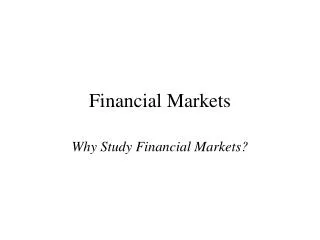
Pareto distribution • The Pareto distribution, named after the Italian economistVilfredo Pareto, is a power lawprobability distribution found in a large number of real-world situations. This distribution is also known, mostly outside economics, as the Bradford distribution. • Pareto originally used this distribution to describe the allocation of wealth among individuals since it seemed to show rather well the way that a larger portion of the wealth of any society is owned by a smaller percentage of the people in that society. This idea is sometimes expressed more simply as the Pareto principle or the "80-20 rule" which says that 20% of the population owns 80% of the wealth.
It can be seen from the PDF graph on the right, that the "probability" or fraction of the population p(x) that owns a small amount of wealth per person (x ) is rather high, and then decreases steadily as wealth increases. This distribution is not just limited to describing wealth or income distribution, but to many situations in which an equilibrium is found in the distribution of the "small" to the "large". The following examples are sometimes seen as approximately Pareto-distributed: • Frequencies of words in longer texts • The size of human settlements (few cities, many hamlets/villages) • File size distribution of Internet traffic which uses the TCP protocol (many smaller files, few larger ones) • Clusters of Bose-Einstein condensate near absolute zero • The value of oil reserves in oil fields (a few large fields, many small fields) • The length distribution in jobs assigned supercomputers (a few large ones, many small ones) • The standardized price returns on individual stocks • Size of sand particles • Size of meteorites • Number of species per genus (please note the subjectivity involved: The tendency to divide a genus into two or more increases with the number of species in it) • Areas burnt in forest fires • Mathematically speaking, if X is a random variable with a Pareto distribution, then the probability distribution of X is characterized by the statement • where x is any number greater than xm, which is the (necessarily positive) minimum possible value of X, and k is a positive parameter. The family of Pareto distributions is parameterized by two quantities, xm and k.