Download
1 / 83
830 likes | 1.34k Views
Results from the 2009 AP Statistics Exam Administration. Allan Rossman, Cal Poly – San Luis Obispo Ruth Carver, Germantown Academy. Outline. Introductions Six questions on operational exam Intent Question Common errors Advice for teachers Overall performance on operational exam

E N D
Results from the 2009 AP Statistics Exam Administration Allan Rossman, Cal Poly – San Luis Obispo Ruth Carver, Germantown Academy
Outline Introductions Six questions on operational exam Intent Question Common errors Advice for teachers Overall performance on operational exam Comparability study Q & A
Introductions • Allan • Chief Reader-Designate for past year • Professor of Statistics at Cal Poly • Ruth • Test Development Committee member • Just completed first year • Math teacher at Germantown Academy (near Philadelphia)
Introductions (cont.) • We represent other TDC members • Ken Koehler (Chair) • Chris Franklin (Chief Reader “Emeritus”) • Dorinda Hewitt • Chris Olsen (CB liaison, now retired from TDC) • Tom Short • Josh Tabor (now retired from TDC) • Bob Taylor • New TDC members • Floyd Bullard, John Mahoney
#1: Intent of question Assess a student’s ability to: construct an appropriate graphical display for comparing the distributions of two categorical variables; summarize from this graph the relationship of the two categorical variables; identify the appropriate statistical procedure to test if an association exists between two categorical variables and stating appropriate hypotheses.
#1: The question A simple random sample of 100 high school seniors was selected from a large school district. The gender of each student was recorded, and each student was asked the following questions. 1. Have you ever had a part-time job? 2. If you answered yes to the previous question, was your part-time job in the summer only?
#1: The question (cont.) The responses are summarized in the table below.
#1: The question- part (a) On the grid below, construct a graphical display that represents the association between gender and job experience for the students in the sample.
#1: Common errors- part (a) Use counts (frequencies) instead of percents (relative frequencies) Not appropriate when comparing groups of unequal size Provide no or incorrect label on vertical axis Indicate conditioning on one variable (say gender), but draw graph as if conditioning on other variable (say job experience). Construct nonstandard graphs of many varieties
#1: The question- part (b) Write a few sentences summarizing what the display in part (a) reveals about the association between gender and job experience for the students in the sample.
#1: Common errors- part (b) Not fully discuss how males and females compare in all three job experience categories. Some only commented on which gender had more (or fewer) part-time jobs, ignoring the two different categories Struggle to communicate statistical thinking clearly when writing sentences about the association between gender and job experience. Describe graphs as if discussing quantitative data, using terms like shape, center, spread, correlation None of these appropriate for describing distributions of categorical data
#1: The question- part (c) Which test of significance should be used to test if there is an association between gender and job experience for the population of high school seniors in the district? State the null and alternative hypotheses for the test, but do not perform the test.
#1: Common errors- part (c) Could not correctly name appropriate test Some incomplete names, like “chi-square test” Some stated hypotheses suggesting causation, not appropriate for observational study Ho: Gender has no effect on job experience. Ha: Gender has an effect on job experience. Several attempted to use symbols to state hypotheses Very hard to do well for chi-square test of association/independence
#1: Advice for teachers Pay attention to categorical variables! Graphical displays: bar graphs Numerical summaries: conditional proportions Cannot over-emphasize distinction between categorical vs. quantitative variables Focus on concept of independence Distribution of one variable (e.g., gender) is identical for all categories of the other (e.g., job condition)
#2: Intent of question Assess a student’s ability to: calculate a percentile value from a normal probability distribution; recognize a binomial scenario and calculate an appropriate probability; use the sampling distribution of the sample mean to find a probability for the mean of five observations.
#2: The question A tire manufacturer designed a new tread pattern for its all-weather tires. Repeated tests were conducted on cars of approximately the same weight traveling at 60 miles per hour. The tests showed that the new tread pattern enables the cars to stop completely in an average distance of 125 feet with a standard deviation of 6.5 feet and that the stopping distances are approximately normally distributed.
#2: Parts (a)-(c) • What is the 70th percentile of the distribution of stopping distances ? • What is the probability that at least 2 cars out of 5 randomly selected cars in the study will stop in a distance that is greater than the distance calculated in part (a) ? • What is the probability that a randomly selected sample of 5 cars in the study will have a mean stopping distance of at least 130 feet ?
#2: The question- part (a) What is the 70th percentile of the distribution of stopping distances?
#2: Common errors- part (a) A number of students set z=0.7 and attempted to calculate the stopping distance. Many had difficulty determining the 70%-tile. Several students interpreted the 70%-tile to be 70% centered about the mean. By doing so, several used the 68-95-99% rule to try to solve the problem. Used “calculator speak” to calculate stopping distance without defining parameters of the distribution. Calculator commands without defining the arguments for the commands are discouraged. Sketches of the approximately normal distribution were unclear and unlabeled.
#2: The question- part (b) What is the probability that at least 2 cars out of 5 randomly selected cars in the study will stop in a distance that is greater than the distance calculated in part (a) ?
#2: Common errors- part (b) Several students failed to use the binomial distribution correctly; calculating 1 - P( Y ≤ 2 ) instead of 1 - P( Y ≤ 1). Several students only gave one term, generally, P(Y=2). Several students used 0.7 as their probability of a success, as well as incorrectly defining the parameters of the binomial distribution Several students constructed another normal probability not seeing the binomial was needed.
#2: The question- part (c) What is the probability that a randomly selected sample of 5 cars in the study will have a mean stopping distance of at least 130 feet?
#2: Common errors- part (c) Several students failed to get the sampling distribution for the sample mean statistic,-didn’t define the distribution or its parameters correctly. Several students gave a value z=1.72, and a value p=0.0427, without correctly indicating that this probability relates to P( Z ≥ 1.72) = 1 - P( Z < 1.72)=0.0427. Several students confused the question with a test of hypothesis and gave the probability P( Z ≥ 1.72) = 1 - P( Z < 1.72)=0.0427 as a p-value.
#2: Advice for teachers Pay attention to the distribution being used and its corresponding parameters. Use standard notation to name the distribution and its corresponding parameters. For example N(125, 6.5) for a Normal Distribution B(5, 0.3) or Bin(5, 0.3) for a Binomial Distribution Avoid calculator-speak such as invNorm(0.70,125,6.5); it is not sufficient for defining a distribution and its parameters. An appropriately labeled sketch with correct labels for center and spread is a definite plus.
#2: Advice for teachers (cont.) Cannot overemphasize the distinction between the distribution of a variable and the sampling distribution of a sample statistic of a variable. Have students define the variable of interest (in words) and the distribution of the variable (using standard notation). For example X = the stopping distance of a car with new tread tires X ~N (125, 6.5) = the mean of the stopping distances of five randomly selected cars.
#3: Intent of question • Assess a student’s ability to: • describe a randomization process required for comparing two groups in a randomized experiment • describe a potential consequence of using self-selection instead of randomization
#3: The question Before beginning a unit on frog anatomy, a seventh-grade biology teacher gives each of the 24 students in the class a pre-test to assess their knowledge of frog anatomy. The teacher wants to compare the effectiveness of an instructional program in which students physically dissect frogs with the effectiveness of a different program in which students use computer software that only simulates the dissection of a frog. After completing one of the two programs, students will be given a posttest to assess their knowledge of frog anatomy. The teacher will then analyze the changes in the test scores (score on the pre-test minus score on posttest).
#3: The question (cont.) (a) Describe a method for assigning the 24 students to two groups of equal size that allows for a statistically valid comparison of the two instructional programs.
#3(a): Common errors • Not stating a specific device or mechanism for randomization • Not specifying groups in context • I.e., forming group 1 and group 2 but not indicating which is the dissection and which is the computer simulation group • Using a stopping rule with a coin toss (or equivalent) without prior randomization • Referring to simple random samples
#3(a): Common errors (cont.) • Providing only a design diagram • Picking names or numbers from a hat but forgetting to first mix the contents • Using a paired design but not blocking on similar pre-test scores • Forming blocks on a characteristic other than pre-test, such as gender
#3: The question (cont.) (b) Suppose the teacher decided to allow the students in the class to select which instructional program on frog anatomy (physical dissection or computer simulation) they prefer to take, and 11 students choose actual dissection and 13 students choose computer simulation. How might that self-selection process jeopardize a statistically valid comparison of the changes in the test scores (score on post-test minus score on pre-test) for the two instructional programs? Provide a specific example to support your answer.
#3(b): Common errors • Stating a reasonable characteristic but only saying that students “like it” • Not describe how behaviors associated with the self-selection criterion impact the changes in the differences (post – pre). • Referring only to the post-test (instead of the change in score)
#3(b): Common errors (cont.) • Mentioning a vague aspect of performance • E.g., do better, learn more/less • Using common terms unclearly • Bias, observation, voluntary response, … • Mentioning only a characteristic without any connection to performance
#3: Advice for teachers • Give practice, feedback in providing enough detail in describing randomization process • So two KSUs (“knowledgeable statistics users”) would use the same method • Make students aware of (subtle) “stopping rule” issue • Can’t just balance groups at end unless order has been randomized to begin with
#3: Advice for teachers (cont.) • Pay attention to what the variables are • Response is change in test score (post – pre) • Emphasize concept of confounding • Challenging concept • Confounding variable must relate to both explanatory and response variables
#4: Intent of question Assess a student’s ability to: identify and compute an appropriate confidence interval, after checking the necessary conditions; interpret the interval in the context of the question; use the confidence interval to make an inference about whether or not a council member’s belief is supported.
#4: The question One of the two fire stations in a certain town responds to calls in the northern half of the town, and the other fire station responds to calls in the southern half of the town. One of the town council members believes that the two fire stations have different mean response times. Response time is measured by the difference between the time an emergency call comes into the fire station and the time the first fire truck arrives at the scene of the fire.
#4: The question (cont.) Data were collected to investigate whether the council member’s belief is correct. A random sample of 50 calls selected from the northern fire station had a mean response time of 4.3 minutes with a standard deviation of 3.7 minutes. A random sample of 50 calls selected from the southern fire station had a mean response time of 5.3 minutes with a standard deviation of 3.2 minutes.
#4: Parts (a)-(b) • Construct and interpret a 95 percent confidence interval for the difference in mean response times between the two fire stations. • Does the confidence interval in part (a) support the council member’s belief that the two fire stations have different mean response times? Explain.
#4: The question- part (a) Construct and interpret a 95 percent confidence interval for the difference in mean response times between the two fire stations.
#4: Common errors- part (a) Many students identified a z confidence interval as the appropriate procedure rather than a t. Many students failed to check the sample sizecondition at all. Some students did an inadequate job of checking the sample size condition by saying that the samples are large enough, with no reference to a number (such as 25 or 30), the central limit theorem or sampling distributions. Some students stated that 50 is large enough to assume that the populations or samples or data are approximatelynormal, rather than that the sampling distribution(s) is (are) approximately normal. Step 1 (name distribution+ conditions)
#4: Common errors- part (a) (cont.) More students received credit for this part than for any of the other parts, but: A few students used1.645 as the multiplier in their computation. A few students neglected to square the standard deviations when computing the standard error, and consequently presented an incorrect finalanswer. A few students thought that the interval could not go below 0, and truncated it at 0. Step 2 (Mechanics)
#4: Common errors- part (a) (cont.) Some students omitted the word “mean” and interpreted the interval as applying to the difference in response times. Some students omitted the word “difference” or similar words to indicate the interval is for a difference in means, stating that the interval is for the “mean response time.” A few students omitted the context. A few students interpreted the confidence level instead of the confidence interval. A few students interpreted the confidence interval correctly but interpreted the confidence level incorrectly. A few students wrote that the confidence interval was for a “mean proportion” or similar wording using “proportion.” Step 3 (Interpretation)
#4: The question- part (b) Does the confidence interval in part (a) support the council member’s belief that the two fire stations have different mean response times? Explain.
#4: Common errors- part (b) Many students made a statistically incorrect statement, such as “because the interval contains 0, the council member’s belief is wrong.” Some students thought that the interval supported the council member’s belief because it included more values on one side of 0 than the other. Some students thought that the interval supported the council member’s belief because it included values as large as 2 minutes. A few students based a conclusion solely on testing hypotheses and made no reference to the confidence interval.
#4: Advice for teachers Pay attention to the parameter of interest Response time/ difference in response times/ mean response time/ difference in mean response times Spiral inference procedures Identify correct procedure from mixed problem set Verification of conditions for a particular procedure Focus on relationship between hypothesis test and corresponding confidence interval Values contained in the interval Contextual meaning beyond the mantra.
#5: Intent of question • Assess a student’s ability to: • interpret a p-value in context • make an appropriate conclusion about the study based on the p-value • based on the conclusion, identify the type of error that could have occurred and a possible consequence of this error in context
#5: The question For many years, the medically accepted practice of giving aid to a person experiencing a heart attack was to have the person who placed the emergency call administer chest compression (CC) plus standard mouth-to-mouth resuscitation (MMR) to the heart attack patient until the emergency response team arrived. However, some researchers believed that CC alone would be a more effective approach.
#5: The question (cont.) In the 1990s a study was conducted in Seattle in which 518 cases were randomly assigned to treatments: 278 to CC plus standard MMR and 240 to CC alone. A total of 64 patients survived the heart attack: 29 in the group receiving CC plus standard MMR, and 35 in the group receiving CC alone. A test of significance was conducted on the following hypotheses.
#5: The question (cont.) H0: The survival rates for the two treatments are equal. Ha: The treatment that uses CC alone produces a higher survival rate. This test resulted in a p-value of 0.0761.