Collisionless Systems

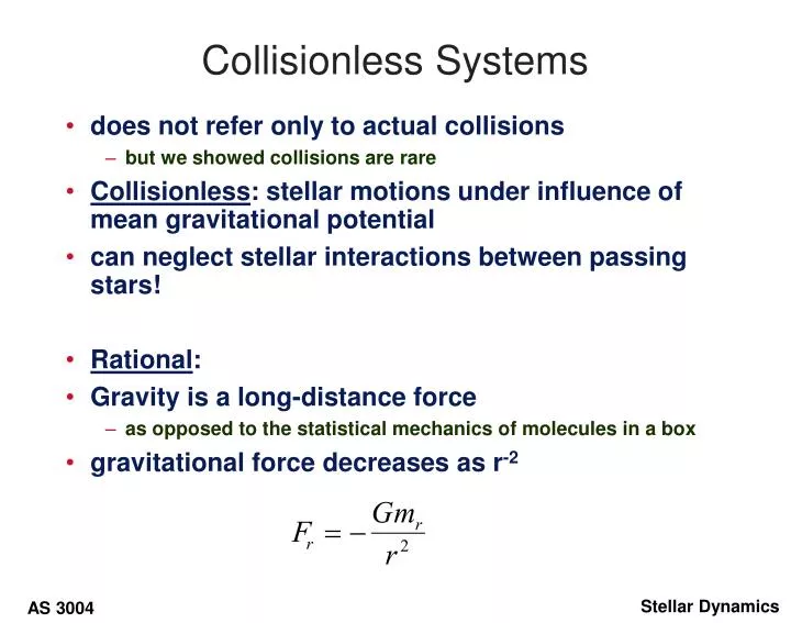
Collisionless Systems • does not refer only to actual collisions • but we showed collisions are rare • Collisionless: stellar motions under influence of mean gravitational potential • can neglect stellar interactions between passing stars! • Rational: • Gravity is a long-distance force • as opposed to the statistical mechanics of molecules in a box • gravitational force decreases as r-2

collisionless systems • total mass at r dependes on number of stars • but number of stars at r is ~ nr r2 • so the net effect is that if the density is uniform, all regions contribute equally. • force determined by gross structure of system! • use smoothed gravitational potential • collisionless no evolution

Stellar interactions • When are interactions important? • Consider a system of N stars or mass m • evaluate deflection of star as it crosses system • consider en encounter with star of mass m at a distance b: • where x = v t x v q b r Fperp

Stellar interactions cont. • the change in the velocity Dvperp is then • using s = vt / b • an easier way of estimating Dvperp is by using impulse approximation: Dvperp = FperpDt • where Fperp is the force at closest approach and • the duration of the interaction can be estimated as : Dt = 2 b / v • using this estimate Dvperp is :

Number of encounters • How many encounters occur at impact parameter b? • let system diameter be: 2R • surface density of stars is ~ N/šR2 • the number encountering within b b + Db is: • each encounter has effect Dvperp but each one randomly oriented • sum is zero: b b+Db

change in kinetic energy • but suming over squares (Dvperp2) is > 0 • hence • now consider encounters over all b • then • but @ b=0, 1/b is infinte! • need to replace lower limit with some bmin • estimate as expected distance of closest approach such that • set by equating kinetic and potential energies

Relaxation time • hence v2 changes by Dv2 each time it crosses the system where Dv2 is: the system is therefore no longer collisionless when v2 ~ Dv2 • which occurs after nrelax times across the system or nrelax crossing times • and thus the relaxation time is:

Relaxation time cont. • can use collisionless approx. only for t < trelax ! • mass segregation occurs on relaxation timescale • also referred to as equipartition • where kinetic energy is mass independent • hence • and the massive stars, with lower specific energy sink to the centre of the gravitational p otential • globular cluster, N=105, R=10 pc • tcross ~ 2 R / v ~ 105 years • trelax ~ 108 years << age of cluster: relaxed • galaxy, N=1011, R=15 kpc • tcross ~ 108 years • trelax ~ 1015 years >> age of galaxy: collisionless • cluster of galaxie: trelax ~ age

Collisionless Systems • stars move under influence of a smooth gravitational potential • determined by overall structure of system • Statistical treatment of motions • collisionless Boltzman equation • Jeans equations • provide link between theoretical models (potentials) and observable quantities. • instead of following individual orbits • study motions as a function of position in system • Use CBE, Jeans to determine mass distributions and total masses

Collisionless Boltzman Equation • for a smooth potential F(x,t) • The number of stars with positions in volume d3x centred on x and with velocities d3v centred on v is: • where is the Distribution Function (DF) or the Phase-Space Density • and everywhere is phase space • Now, for a stellar system, if we know the phase-space density at time t0, then we can predict it at any subsequent time

motions in phase-space • Flow of points in phase space corresponding to stars moving along their orbits. • phase space coords: • and the velocity of the flow is then: • where is the 6-D vector related to in the same way the 3-D velocity vector relates to x • stars are conserved in this flow, with no encounters, stars do not jump from one point to another in phase space. • they drift slowly through phase space

fluid analogy • regard stars as making up a fluid in phase space with a phase space density • assume that is a smooth function, continuous and differentiable • good for N 105 • as in a fluid, we have a continuity equation • fluid in box of volume V, density r, and velocity v, the change in mass is then: • using the divergence theorem:

continuity equation • must hold for any volume V, hence: • in same, manner, density of stars in phase space obeys a continuity equation: • If we integrate over a volume of phase space V, then we see that the first term is the rate of change of the stars in V, while the second term is the rate of outflow/inflow of stars from/into V. • as in the fluid case • note: • ind. variables, x,v, and grad of pot ind. of v! 0

Collisionless Boltzmann Equation • Hence, we can simplify the continuity equation to the CBE: • or • in vector notation • notice that in the event of stellar encounters, then differs significantly from that given by • no longer collisionless • require additional terms in equation

CBE cont. • can define a Lagrangian derivative • Lagrangian flows are where the coordinates travel along with the motions (flow) • hence x= x0 = constant for a given star • then we have: • and • rate of change of phase space density seen by observer travelling with star • the flow of stellar phase points through phase space is incompressible • f around the phase point of a given star remains the same

incompressible flow • example of incompressible flow • idealised marathon race • each runner runs at constant speed • At start • the number density of runners is large, but they travel at wide variety of speeds • At finish • the number density is low, but at any given time the runners going past have nearly the same speed

The Jeans Equations • The DF (phase space density f) is a function of 7 variables and hence generally difficult to solve • Can gain insights by taking moments of the equation. • from the CBE: • then integrate over all possible velocities • where the summation over subscripts is implicit

Jeans equations cont. • simplify • first term: velocity range doesn’t depend on time, hence we can take partial w.r.t. time outside • second term, vi does not depend on xi, so we can take partial w.r.t xi outside • third term: apply divergence theorem so that • but at very large velocities, f 0, hence last term is zero • must be true for all bound systems

First Jeans equation • define spatial density of stars n(x) • and the mean stellar velocity v(x) • then our first (zeroth) moment equation becomes • this is the first Jeans equation • analogous to the continuity equation for a fluid.

Second Jeans equation • multiply the CBE by vj and then integrate over all velocities • taking the integrand from the third term • but from the divergence theorem • and thus B

2nd Jeans equations cont. • now, clearly the term except where i=j where it is =1 • hence we replace differential with the Kroneker delta function dij (=0 when i°j, =1 when i=j) • we can also define: • and thus we can rewrite B as: • the second Jeans equation!

3rd Jeans equation • now, take the last equation and subtract vj times the continuity equation (1st Jeans equation) • ie • which yields: • we can separate into a part that is due to the streaming motions and a part that arises because the stars near any given point x do not have all the same velocity. ie, a velocity dispersion gives a measure of the velocity dispersion in various directions C

3rd Jeans Equation • then C becomes: • This equation, the third Jeans equation, is very similar to the Euler equation for a fluid flow: • both LHS are of the same form, as are the first terms on the RHS thus it follows that the last term must represent some sort of pressure force

Stress Tensor • Hence if we associate: then the quantity is called the Stress Tensor • it describes a pressure which is anisotropic • not the same in all directions • and we can refer to a “pressure supported” system • the tensor is symmetric, as seen from the definition of • therefore we can chose a set of orthogonal axes such that the tensor is diagonal • ellipsoid with these axes, and semi-major axes given by the is called the Velocity Ellipsoid

Jeans Equations • So, we have the three Jeans equations, first applied to stellar dynamics by Sir James Jeans • again: the continuity equation the (first) Jeans eq. the “Euler- flow” eq. • these equations link observable quantities to potential gradients which describe the mass distribution in a system. • can be applied to many diverse problems of stellar dynamics

Jeans Equation • Compact form, s=x, y, z, R, r, … • e.g., oblate spheroid, s=[R,phi,z], • Isotropic rotator, a=[-Vrot^2/R, 0, 0], sigma=sigma_s • Tangential anisotropic (b<0), a=[b*sigma^2)/R, 0, 0], sigma=sigma_R=sigma_z=sigma_phi/(1-b), • e.g., non-rotating sphere, s=[r,th,phi], a=[-2*b*sigma_r^2/r, 0, 0], sigma_th=sigma_phi=(1-b)*sigma_r

Applications of the Jeans Equations • I. The mass density in the solar neighbourhood • Using velocity and density distribution perpendicular to the Galactic disc • cylindrical coordinates • Multiply CBE by vz and integrate over all velocities to obtain: • compare observed and predicted number-density and velocity distributions as a function of height Z above Galactic disc • assume steady state so drop first term

mass desnity of solar neighbourhood cont. • 2nd and 4th terms contain • For small z/R, we find that • hence these terms are (z/R)2 smaller than the first and fifth terms • in the solar neighbourhood, R~8.5 kpc, |z|< 1kpc, these terms can be neglected. • Hence, Jeans equation reduces to:

mass density in solar neighbourhood • Using Poisson’s equation in cylindrical coordinates: • for axisymmetric systems • and density a function of R,z, so • where the radial force, • Near z=0, the second term on the LHS is relatively small, so can be neglected.

mass density cont. • Poisson’s equation then reduces to • and we can then replace the potential in the Jeans equation as • all quantities on the LHS are, in principle, determinable from observations. • Hence we can determine local mass density r = r0 • Known as the Oort limit • difficult due to double differentiation!

local mass density • Don’t need to calculate for all stars • just a well defined population (ie G stars, BDs etc) • test particles (don’t need all the mass to test potential) • Procedure • determine the number density n, and the mean square vertical velocity, vz2, the variance of the square of the velocity dispersion in the solar neighbourhood. • need a reliable “tracer population” of stars • whose motions do not reflect formation • hence old population that has orbited Galaxy many times • ages > several x 109 years • N.B. problems of double differentiation of the number density n derived from observations • need a large sample of stars to obtain vz as f(z) • ensure that vz is constant in time • ie stars have forgotten initial motion

local mass density • > 1000 stars required • Oort : r0 = 0.15 Msol pc-3 • K dwarf stars (Kuijken and Gilmore 1989) • MNRAS 239, 651 • Dynamical mass density of r0 = 0.11 Msol pc-3 • also done with F stars (Knude 1994) • Observed mass density of stars plus interstellar gas within a 20 pc radius is r0 = 0.10 Msol pc-3 • can get better estimate of surface density • out to 700 pc S ~ 90 Msol pc-2 • from rotation curve Srot ~ 200 Msol pc-2

Application II • Velocity dispersions and masses in spherical systems • For a spherically symmetric system we have • a non-rotating galaxy has • and the velocity ellipsoids are spheroids with their symmetry axes pointing towards the galactic centre • If we define b as • the degree of anisotropy of the velocity dispersion

spherical systems cont. • then the Jeans equation is: • Need observations to determine , vr and b as a function of radius r for a stellar population in a galaxy • then, with • and the circular speed

Mass of spherical systems • we can use this equation to establish the total mass (and as a function of radius) for a spherical galaxy • including any unseen halo • Example 1) globular clusters and satellite galaxies around major galaxies • within 150 kpc • Need n(r), vr2, b to find M(r) • Several attempts for Milky Way • all suffer from problem of small numbers • N ~ 15

Mass of the Milky Way • Little and Tremaine tried two extreme values of b • Isotropic orbits: • Radial orbits • If we assume a power law for the density distribution • then we obtain

Mass of the Milky Way • Drop first term, we have solutions • E.g., Point mass a=0, Tracer gam=3.5, Isotro b = 0 : • E.g. Flat rotation a=1, Self-grav gamma=2, Radial anis. b >0 : • For the isotropic case, Little and Tremaine determined a TOTAL mass of 2.4 (+1.3, -0,7) 1011 Msol • 3 times the disc and spheroidal mass

Collisionless Systems