Download

1 / 25
260 likes | 358 Views
Unit 4: Regression assumptions: Evaluating their tenability. The S-030 roadmap: Where’s this unit in the big picture?. Unit 1: Introduction to simple linear regression. Unit 2: Correlation and causality. Unit 3: Inference for the regression model. Building a solid foundation.

E N D
The S-030 roadmap: Where’s this unit in the big picture? Unit 1: Introduction to simple linear regression Unit 2: Correlation and causality Unit 3: Inference for the regression model Building a solid foundation Unit 5: Transformations to achieve linearity Unit 4: Regression assumptions: Evaluating their tenability Mastering the subtleties Adding additional predictors Unit 6: The basics of multiple regression Unit 7: Statistical control in depth: Correlation and collinearity Generalizing to other types of predictors and effects Unit 9: Categorical predictors II: Polychotomies Unit 8: Categorical predictors I: Dichotomies Unit 10: Interaction and quadratic effects Pulling it all together Unit 11: Regression modeling in practice
In this unit, we’re going to learn about… • Reprise of the assumptions required for least squares estimation and inference • The four major types of model violations: • Outliers • Nonlinearity • Heteroscedasticity • Non-independence of errors • Determining whether the regression assumptions hold—strategies and rationale • Why residuals provide a powerful lens for evaluating regression assumptions • Residuals as controlled observations • Raw residuals and studentized residuals • Residual plots: How to construct them and what to look for • What should we do if we find an outlier or other unusual observation? • How would we summarize our results?
(Reprise of) Assumptions required for least squares estimation & inference Y Y|x3 Y|x2 Y|x1 X … x1 x2 x3 • At each value of X, there is a distribution of Y. These distributions have a mean µY|X and a variance of σ2Y|X • The straight line model is correct. The means of each of these distributions, the µY|X‘s, may be joined by a straight line. • Homoscedasticity. The variances of each of these distributions, the σ2Y|X’s, are identical. • Independence of observations. • At each given value of X (at each xi), the values of Y (the yi’s) are independent of each other. 5.Normality. At each given value of X (at each xi), the values of Y (the yi’s) are normally distributed Assumptions ARE NOT about the sample, X, or Y overall. Assumptions ARE about the behavior of Y at each X in the population
Anscombe’s data: Good looks can be deceiving Data Set III x y 10 7.46 8 6.77 13 12.74 9 7.11 11 7.81 14 8.84 6 6.08 4 5.39 12 8.15 7 6.42 5 5.73 Data Set I x y 10 8.04 8 6.95 13 7.58 9 8.81 11 8.33 14 9.96 6 7.24 4 4.26 12 10.84 7 4.82 5 5.68 Data Set IV x y 8 6.58 8 5.76 8 7.71 8 8.84 8 8.47 8 7.04 8 5.25 8 5.56 8 7.91 8 6.89 19 12.50 Data Set II x y 10 9.14 8 8.14 13 8.74 9 8.77 11 9.26 14 8.10 6 6.13 4 3.10 12 9.13 7 7.26 5 4.74
Four major types of model violations Heteroscedasticity. The variance of Y varies as a function of X Nonlinearity. There’s a relationship between Y and X, but it’s not best summarized by a straight line Outliers. Extreme observations that don’t fit the general pattern Non-independence of errors. Observations within the data set are clustered (or otherwise related)** A cautionary tale…. **Remember we can’t see this one visually
Where to go for dinner? Using Zagat ratings to identify restaurants that are “good” and “poor” values Predictor Outcome The UNIVARIATE Procedure Variable: COST Location Variability Mean 38.52632 Std Deviation 10.54574 Median 38.00000 Variance 111.21263 Mode 38.00000 Range 50.00000 The UNIVARIATE Procedure Variable: RATING Location Variability Mean 20.98684 Std Deviation 2.49589 Median 21.00000 Variance 6.22945 Mode 19.66667 Range 9.33333 Stem Leaf # Boxplot 68 0 1 0 66 64 0 1 | 62 0 1 | 60 | 58 0 1 | 56 0 1 | 54 00 2 | 52 000 3 | 50 0000 4 | 48 | 46 00 2 | 44 00000 5 +-----+ 42 00000 5 | | 40 000 3 | | 38 0000000000 10 *--+--* 36 0000 4 | | 34 000000 6 | | 32 0000 4 | | 30 0000000 7 +-----+ 28 000000 6 | 26 00000 5 | 24 000 3 | 22 0 1 | 20 | 18 0 1 | ----+----+--- Stem Leaf # Boxplot 25 777 3 | 25 333 3 | 24 | 24 0000033 7 | 23 7777 4 | 23 03 2 | 22 777 3 +-----+ 22 0000333 7 | | 21 7 1 | | 21 000003333 9 *--+--* 20 777 3 | | 20 00033 5 | | 19 77777 5 | | 19 0003333 7 +-----+ 18 777 3 | 18 00333 5 | 17 777 3 | 17 00033 5 | 16 | 16 3 1 | ----+----+----+----+ Residuals as “controlled” observations n = 76 NAME COST RATING Jacob Wirth 26 16.3333 Grafton St. Pub 24 17.0000 29 Newbury 38 17.0000 Vox Populi 31 17.0000 Avenue One 35 17.3333 Orleans 28 17.3333 Daedalus 26 17.6667 ... 224 Boston St. 31 21.3333 West Side Lounge 30 21.3333 Fava 43 21.6667 ... Harvest 46 23.6667 Square Café 39 23.6667 Troquet 54 23.6667 TW Foods 39 24.0000 flora 40 24.0000 ... Hamersley's 56 25.3333 Icarus 54 25.3333 Excelsior 65 25.6667 Federalist 69 25.6667 Meritage 63 25.6667 RQ: Do you get what you pay for?:What’s the relationship between a restaurant’s rating and its cost? RQ: Which restaurants are good values?:Given what you’re paying (controlling for price), where do you get the best food?
What’s the relationship between cost and restaurant ratings? Effect is strong: 61.6% of the variation in ratings is associated with cost The REG Procedure Dependent Variable: RATING Analysis of Variance Sum of Mean Source DF Squares Square Model 1 287.86080 287.86080 Error 74 179.34826 2.42363 Corrected Total 75 467.20906 Root MSE 1.55680 R-Square 0.6161 Dependent Mean 20.98684 Adj R-Sq 0.6109 Coeff Var 7.41798 Parameter Estimates Parameter Standard Variable DF Estimate Error t Value Pr > |t| Intercept 1 13.82968 0.68057 20.32 <.0001 COST 1 0.18577 0.01705 10.90 <.0001 Estimated effect is quite precise: Narrow 95% CI (0.1523, 0.2193) Estimated effect is large†: Each $10.00 difference in cost is positively associated with a 1.9 difference in ratings Effect is statistically significant: Unlikely that in the population of Boston restaurants, there’s no relationship between price & ratings †How large is large? Compare to SD of outcome (≈ 2.5)
How can we determine whether the assumptions hold? ^ -Y Y Y Y|x3 Y|x2 Y|x1 X X … x1 x2 x3 … x1 x2 x3 0 What does it mean to refer to the “values of Y at each X?” residuals • Assumptions we can examine: • Normality • Homoscedasticity • Linearity • which all refer to the values of Y at each X • So the residual distributions should be: • Normal • Homoscedastic • Totally unrelated to X Go to Put Points The hope? To see random scatter in the residual plot
A first look at residuals for the restaurant data Dependent Predicted Obs NAME Variable Value Residual 6 Bambara 20.6667 21.6322 -0.9655 7 Birch St. Bistro 19.3333 19.4029 -0.0695 8 Blarney Stone 18.3333 17.9167 0.4166 9 blu 23.6667 23.3041 0.3625 10 Brenden Crocker' 22.0000 20.7033 1.2967 11 Bristol 25.3333 22.1895 3.1439 12 B-Side Lounge 18.6667 18.6598 0.006881 13 Central Kitchen 20.0000 17.3594 2.6406 14 Daedalus 17.6667 18.6598 -0.9931 15 Dalia's Bistro 18.0000 19.5887 -1.5887 16 Dalya's 21.0000 21.0748 -0.0748 17 Dedo Lounge 19.6667 20.1460 -0.4793 18 Devlin's 20.3333 18.4740 1.8593 19 Excelsior 25.6667 25.9049 -0.2383 20 Fava 21.6667 21.8179 -0.1513 21 Federalist 25.6667 26.6480 -0.9814 22 flora 24.0000 21.2606 2.7394 23 Franklin Café 21.0000 19.7744 1.2256 24 Gardner Museum 19.0000 18.4740 0.5260 25 Gargoyles 22.6667 20.7033 1.9634 26 Grafton St. Pub 17.0000 18.2882 -1.2882 27 Grapevine 22.6667 20.8891 1.7776 28 Green St. Grill 19.3333 19.0313 0.3020 29 Hamersley's Bist 25.3333 24.2330 1.1003 30 Harvest 23.6667 22.3753 1.2914 . . . 57 Square Café 23.6667 21.0748 2.5918 58 Stanhope Grille 18.6667 21.8179 -3.1513 59 Stephanie's 18.6667 19.9602 -1.2935 60 Temple Bar 17.6667 18.8456 -1.1789 61 Ten Tables 23.0000 20.8891 2.1109 62 33 Restaurant 19.3333 21.6322 -2.2988 63 Top of the Hub 22.0000 23.1183 -1.1183 64 Tremont 647 19.6667 20.3317 -0.6651 65 Troquet 23.6667 23.8614 -0.1948 66 Tryst 20.6667 21.2606 -0.5939 67 29 Newbury 17.0000 20.8891 -3.8891 The UNIVARIATE Procedure Variable: rawres1 (Residual) Basic Statistical Measures Location Variability Mean 0.000000 Std Deviation 1.54639 Median 0.001587 Variance 2.39131 Mode . Range 7.03292 Interquartile Range 2.14756 Stem Leaf # Boxplot 3 1 1 | 2 6679 4 | 2 0013 4 | 1 57899 5 | 1 00112334 8 +-----+ 0 5566778 7 | | 0 011133344 9 *--+--* -0 443222110 9 | | -0 977665 6 | | -1 33322110000 11 +-----+ -1 765 3 | -2 3311 4 | -2 65 2 | -3 20 2 | -3 9 1 | ----+----+----+----+ positive negative
What would the residuals look like if they were normally distributed?Introducing studentized residuals 67% 1 3 stdres > 2 is well within our expectations when n= 76 95% (1.96) -4 -3 -2 -1 0 +1 +2 +3 +4 99% ( 2.58) The UNIVARIATE Procedure Variable: stdres (Studentized Residual) Basic Statistical Measures Location Variability Mean -0.00016 Std Deviation 1.00425 Median 0.00105 Variance 1.00852 Mode . Range 4.55280 Interquartile Range 1.40607 Stem Leaf # Boxplot 20 4 1 | 18 9 1 | 16 857 3 | 14 6 1 | 12 25786 5 | 10 35 2 | 8 4437 4 | 6 67239 5 +-----+ 4 1353 4 | | 2 0147346 7 | | 0 08997 5 *-----* -0 630550 6 | + | -2 81961 5 | | -4 7530 4 | | -6 97307652 8 +-----+ -8 9644 4 | -10 13 2 | -12 97 2 | -14 29 2 | -16 83 2 | -18 4 1 | -20 4 1 | -22 | -24 1 1 | • Rule of thumb: If studentized residuals are normally distributed, we expect: • 5% > 2 • 1% > 2.5 • Flag & examine stdres > 2
Do we see anything usual in the residual plots for the restaurant data? Bristol TWFoods flora Bristol Central Kitchen TWFoods Central Kitchen Square Cafe flora Square Cafe Jer ne Vox Populi Jer ne Vox Populi Avenue One Stanhope Grille Avenue One Stanhope Grille 29 Newbury 29 Newbury Raw residuals Studentized residuals 5 best places to eat (controlling for cost) NAME COST RATING RESIDUAL Square Café 39 23.6667 2.59183 Central Kitchen 19 20.0000 2.64063 flora 40 24.0000 2.73939 TWFoods 39 24.0000 2.92516 Bristol 45 25.3333 3.14385 5 most over-rated (controlling for cost) NAME COST RATING RESIDUAL Jer-Ne 52 21.0000 -2.48989 Vox Populi 31 17.0000 -2.58865 Avenue One 35 17.3333 -2.99841 Stanhope Grille 43 18.6667 -3.15127 29 Newbury 38 17.0000 -3.88907
Could (would?) we have spotted these observations on the scatterplot? Bristol • TWFoods flora CentralKitchen Bristol Square Cafe • • • TWFoods flora SquareCafe • Jer ne • CentralKitchen • Stanhope Grille • • Avenue One • 29 Newbury Vox Populi Raw residuals Where were these on the original scatterplot? Jerne Vox Populi Avenue One Stanhope Grille 29 Newbury 5 best places to eat (controlling for cost) NAME COST RATING RESIDUAL Square Café 39 23.6667 2.59183 Central Kitchen 19 20.0000 2.64063 flora 40 24.0000 2.73939 TWFoods 39 24.0000 2.92516 Bristol 45 25.3333 3.14385 5 most over-rated (controlling for cost) NAME COST RATING RESIDUAL Jer-Ne 52 21.0000 -2.48989 Vox Populi 31 17.0000 -2.58865 Avenue One 35 17.3333 -2.99841 Stanhope Grille 43 18.6667 -3.15127 29 Newbury 38 17.0000 -3.88907 Boston Restaurant Weeks, March 9th – 14th & 16th to 21st Three-course Prix-fixe Lunch Menu: $20.08Three-course Prix-fixe Dinner Menu: $33.08
Did the butterfly ballot affect the 2000 Presidential race in Florida? If you punch the second hole, you are voting for the Reform party (ie, Pat Buchanan) Although Democrats are listed second in the left hand column, you vote Democratic by punching the third hole Poly-CY, Internet Resources for political science has much more information on the statistical analysis of the 2000 Presidential election results Of the nearly 6 million votes cast in Florida, the official tally has Bush beating Gore by 537 votes RQ: In the 2000 Presidential election, did Buchanan get more votes than we “would have expected?”
Did Buchanan receive more votes than expected in Palm Beach county? Pinellas Hillsborough Broward, Duvall ID COUNTY BUCH REGREF 1 ALACHUA 262 91 2 BAKER 73 4 3 BAY 248 55 4 BRADFORD 65 3 5 BREVARD 570 148 6 BROWARD 789 332 . . . 48 ORANGE 446 199 49 OSCEOLA 145 62 50 PALM BEACH 3407 337 51 PASCO 570 167 52 PINELLAS 1010 425 . . . 64 VOLUSIA 396 176 65 WAKULLA 46 7 66 WALTON 120 22 67 WASHINGTON 88 9 The UNIVARIATE Procedure Variable: BUCH Location Variability Mean 258.6119 Std Deviation 449.48775 Median 114.0000 Variance 202039 Mode 29.0000 Range 3398 n = 67 Stem Leaf # Boxplot 34 1 1 * 32 30 28 26 24 22 20 18 16 14 12 10 1 1 0 8 4 1 0 6 59 2 0 4 05046677 8 | 2 345677789011 12 +--+--+ 0 112233333333444455677788999900011122245899 42 *-----* ----+----+----+----+----+----+----+----+-- Multiply Stem.Leaf by 10**+2 10 Nov 2000: “The Bush campaign claims that the number of votes for Buchanan in Palm Beach County is perfectly accurate. ‘New information has come to our attention that puts in perspective the results of the vote in Palm Beach County,’ Bush spokesman Ari Fleischer said on Thursday. ‘Palm Beach County is a Pat Buchanan stronghold and that's why Pat Buchanan received 3,407 votes there.’” (Salon.com) View Article
Is Palm Beach county a Buchanan (and Reform party) stronghold? Effect is strong: 55.6% of the variation in Buchanan votes is associated with Reform party registration Palm Beach Estimated effect is somewhat precise: 95% CI (2.87, 4.50) Estimated effect is large: Each registered Reform party member is associated with 3.69 votes for Buchanan Effect is statistically significant: Unlikely that in the population of Florida counties, there’s no relationship between reform party registration and Buchanan votes The REG Procedure Dependent Variable: BUCH Analysis of Variance Sum of Mean Source DF Squares Square Model 1 7412114 7412114 Error 65 5922476 91115 Corrected Total 66 467.20906 Root MSE 301.85265 R-Square 0.5559 Dependent Mean 258.61194 Adj R-Sq 0.5490 Coeff Var 116.72031 Parameter Estimates Parameter Standard Variable DF Estimate Error t Value Pr > |t| Intercept 1 1.53252 46.60847 0.03 0.9739 REGREF 1 3.68671 0.40876 9.02 <.0001
Buchanan stronghold or very unusual data point? 10 Nov 2000: When asked about the Bush campaign's statement, Buchanan's Florida coordinator, Jim McConnell, responded: "That's nonsense.“ He estimate[s] the number of Buchanan activists in the county to be between 300 and 500 -- nowhere near the 3,407 who voted for him. (Salon.com) View Article Palm Beach
What happens if we set aside Palm Beach County? Marion Duval Polk Collier 1106 646 R2=86.4%
How would we summarize the results of this analysis? Palm Beach All Florida counties Without Palm Beach It’s déjà vu all over again… The results of the 2006 congressional elections in Florida The New York Times, 24 February 2007
Decisions about just a few data points can have serious consequences
What’s the big takeaway from this unit? • Regression models invoke a series of important assumptions • Before accepting a set of regression results, you should examine the assumptions to make sure they’re tenable • The assumptions may well be reasonable but you can’t be sure your conclusions are correct unless you have evaluated their tenability • Residuals are the key to evaluating regression assumptions • Regression as statistical control • We often want to do more than just summarize the relationship between variables • Regression provides a straightforward strategy that allows us to statistically control for the effects of a predictor and see what’s “left over” • Residuals can be easily interpreted as “controlled observations” • Outliers can distort regression results or be interesting on their own • Always inspect scatterplots and residual plots to determine whether there are any unusual values that might unduly influence the fitted regression line • If you find outliers, re-fit the regression model without those observations and compare the results • Regardless of how you decide to handle the presence of outliers, always tell your audience about their existence and what you did about them
Appendix: Annotated PC-SAS Code for Unit 4, ZAGAT data proc sortsorts the newly created SAS data set (named “one”). The by statement identifies the variable according to which to data is sorted proc regallows you to add a plot statementthat produces a bivariate scatterplot of the raw and studentized residuals by the predictor (“residual” stands for raw residuals, and “student” for studentized). The syntax is identical to that of proc gplot (ie, plot y*x), (note the “.” after naming the residual, as part of the PLOT statement). The output statement creates a new (temporary) dataset, called RESDAT, that contains all the data in ONE as well as the raw and standardized residuals. proc univariatecan be used tp analyze the new dataset RESDAT andpresents summary statistics of the residuals (e.g., means, sd’s, stem-and-leaf displays). As in any proc univariate, the var statement specifies the residuals you want analyzed; the id statementprovides identifiers for extreme values Note that the handouts include only annotations for the new additional SAS code. For the complete program, check program “Unit 4—ZAGAT analysis” on the website. *------------------------------------------------------* Sorting observations in sample from lowest to highest RATING *------------------------------------------------------*; procsort data=one; by rating; procreg data=one; title2 "Examining residuals from the regression of Rating on Cost"; model rating=cost/p; plot residual.*cost; plot student.*cost; output out=resdat r=rawres student=stdres; id name; *--------------------------------------------------------* Univariate summary information on raw and studentized residuals from OLS regression model RATING on COST *-------------------------------------------------------*; procunivariate data=resdat plot; title2 "Distribution of residuals from the regr of Rating on Cost"; var rawres stdres; id name;
Appendix: Annotated PC-SAS Code for Unit 4, FLVOTE data The datastep here creates a new dataset called “two.” The if-then-delete statement specifies which data points to delete. proc reghere reads the data from the new dataset “two”. An option has been added to the model statement to produce 95% prediction intervals for individuals levels of Y at each value of X (/conf95), superimposed on the bivariate scatterplot. The other plot statement produces a bivariate scatterplot of studentized residuals by predictor. Finally, the output statement creates a new (temporary) dataset, called RESDAT2, that includes all the data in ONE and the raw and standardized residuals. proc univariateanalyzes the new dataset RESDAT2 andpresents summary statistics of the residuals *---------------------------------------------------------------------* Creating FLVote data subset that excludes Palm Beach County (id=50) *----------------------------------------------------------------*; data two; set one; if id=50 then delete; *---------------------------------------------------------------------* Fitting OLS regression model BUCH on REGREF, excluding Palm Beach County Plotting BUCH vs REGREF with 95% prediction interval bands Plotting studentized residuals on REGREF *-------------------------------------------------------------------*; procreg data=two; title2 "Regression results and residual analysis"; model buch=regref/p; plot buch*regref/pred95; plot student.*regref; output out=resdat2 r=residual student=student; id county; *-------------------------------------------------------------------* Univariate summary information of studentized residuals from OLS regression model BUCH on REGREF, excluding Palm Beach County *-------------------------------------------------------------------*; procunivariate data = resdat2 plot; title2 "Studentized Residuals"; var student; id county;
Glossary terms included in Unit 4 • Assumptions • Homoscedasticity • Independence of observations • Linearity • Normality • Outlier • Studentized residuals