Download
1 / 137
1.37k likes | 1.51k Views
Processor Technology. Embedded System HW. Processor Technology. General Purpose (“software”) Application Specific Single Purpose (“Hardware”) IC technology Full Custom/VLSI Semi-custom ASIC (gate-array, standard cell) PLD. Custom single-purpose processors: “ Hardware ”. Outline.

E N D
Processor Technology Embedded System HW
Processor Technology • General Purpose (“software”) • Application Specific • Single Purpose (“Hardware”) • IC technology • Full Custom/VLSI • Semi-custom ASIC (gate-array, standard cell) • PLD
Outline • Introduction • Combinational logic • Sequential logic • Custom single-purpose processor design • RT-level custom single-purpose processor design * Read chapter 2 in “Embedded System Design: A unified Hardware/Software Introduction,” Frank Vahid and Tony Givargis.
Digital camera chip CCD CCD preprocessor Pixel coprocessor D2A A2D lens JPEG codec Microcontroller Multiplier/Accum DMA controller Display ctrl Memory controller ISA bus interface UART LCD ctrl Introduction • Processor • Digital circuit that performs a computation tasks • Controller and datapath • General-purpose: variety of computation tasks • Single-purpose: one particular computation task • Custom single-purpose: non-standard task • A custom single-purpose processor may be • Fast, small, low power • But, high NRE, longer time-to-market, less flexible
… … external control inputs external data inputs controller datapath … … registers datapath control inputs next-state and control logic controller datapath datapath control outputs functional units state register … … external control outputs external data outputs … … a view inside the controller and datapath controller and datapath Custom single-purpose processor basic model
!1 1: (a) black-box view 1 !(!go_i) 2: !go_i x_i GCD go_i y_i 2-J: 3: x = x_i d_o 4: y = y_i !(x!=y) 5: x!=y 6: x<y !(x<y) y = y -x x = x - y 7: 8: 6-J: 5-J: d_o = x 9: 1-J: Example: greatest common divisor • First create algorithm • Convert algorithm to “complex” state machine • Known as FSMD: finite-state machine with datapath • Can use templates to perform such conversion (c) state diagram (b) desired functionality 0: int x, y; 1: while (1) { 2: while (!go_i); 3: x = x_i; 4: y = y_i; 5: while (x != y) { 6: if (x < y) 7: y = y - x; else 8: x = x - y; } 9: d_o = x; }
Assignment statement Loop statement Branch statement a = b next statement while (cond) { loop-body- statements } next statement if (c1) c1 stmts else if c2 c2 stmts else other stmts next statement !cond a = b C: C: c1 !c1*!c2 !c1*c2 cond next statement c1 stmts c2 stmts others loop-body- statements J: J: next statement next statement State diagram templates
!1 1: 1 !(!go_i) 2: x_i y_i !go_i Datapath 2-J: x_sel n-bit 2x1 n-bit 2x1 3: x = x_i y_sel x_ld 0: x 0: y 4: y = y_i y_ld !(x!=y) 5: != < subtractor subtractor x!=y 5: x!=y 5: x!=y 6: x<y 8: x-y 7: y-x 6: x_neq_y x<y !(x<y) x_lt_y 9: d y = y -x x = x - y 7: 8: d_ld d_o 6-J: 5-J: d_o = x 9: 1-J: Creating the datapath • Create a register for any declared variable • Create a functional unit for each arithmetic operation • Connect the ports, registers and functional units • Based on reads and writes • Use multiplexors for multiple sources • Create unique identifier • for each datapath component control input and output
!1 go_i 1: Controller !1 1 !(!go_i) 1: 0000 2: 1 !(!go_i) 0001 2: x_i y_i !go_i !go_i Datapath 2-J: 0010 2-J: x_sel n-bit 2x1 n-bit 2x1 3: x = x_i x_sel = 0 x_ld = 1 0011 3: y_sel x_ld 0: x 0: y 4: y = y_i y_sel = 0 y_ld = 1 y_ld 0100 4: !(x!=y) 5: !x_neq_y 0101 5: != < subtractor subtractor x!=y x_neq_y 5: x!=y 5: x!=y 6: x<y 8: x-y 7: y-x 6: 0110 6: x_neq_y x<y !(x<y) x_lt_y !x_lt_y x_lt_y 9: d y = y -x x = x - y y_sel = 1 y_ld = 1 x_sel = 1 x_ld = 1 7: 8: 7: 8: d_ld 0111 1000 d_o 6-J: 1001 6-J: 5-J: 1010 5-J: d_o = x 9: d_ld = 1 1011 9: 1-J: 1100 1-J: Creating the controller’s FSM • Same structure as FSMD • Replace complex actions/conditions with datapath configurations
x_i y_i (b) Datapath x_sel n-bit 2x1 n-bit 2x1 y_sel x_ld 0: x 0: y y_ld != < subtractor subtractor Controller implementation model 5: x!=y 5: x!=y 6: x<y 8: x-y 7: y-x go_i x_neq_y x_sel Combinational logic y_sel x_lt_y 9: d x_ld d_ld y_ld d_o x_neq_y x_lt_y d_ld Q3 Q2 Q1 Q0 State register I3 I2 I1 I0 Splitting into a controller and datapath go_i Controller !1 1: 0000 1 !(!go_i) 0001 2: !go_i 0010 2-J: x_sel = 0 x_ld = 1 0011 3: y_sel = 0 y_ld = 1 0100 4: x_neq_y=0 0101 5: x_neq_y=1 0110 6: x_lt_y=1 x_lt_y=0 y_sel = 1 y_ld = 1 x_sel = 1 x_ld = 1 7: 8: 0111 1000 1001 6-J: 1010 5-J: d_ld = 1 1011 9: 1100 1-J:
Inputs Outputs Q3 Q2 Q1 Q0 x_neq_y x_lt_y go_i I3 I2 I1 I0 x_sel y_sel x_ld y_ld d_ld 0 0 0 0 * * * 0 0 0 1 X X 0 0 0 0 0 0 1 * * 0 0 0 1 0 X X 0 0 0 0 0 0 1 * * 1 0 0 1 1 X X 0 0 0 0 0 1 0 * * * 0 0 0 1 X X 0 0 0 0 0 1 1 * * * 0 1 0 0 0 X 1 0 0 0 1 0 0 * * * 0 1 0 1 X 0 0 1 0 0 1 0 1 0 * * 1 0 1 1 X X 0 0 0 0 1 0 1 1 * * 0 1 1 0 X X 0 0 0 0 1 1 0 * 0 * 1 0 0 0 X X 0 0 0 0 1 1 0 * 1 * 0 1 1 1 X X 0 0 0 0 1 1 1 * * * 1 0 0 1 X 1 0 1 0 1 0 0 0 * * * 1 0 0 1 1 X 1 0 0 1 0 0 1 * * * 1 0 1 0 X X 0 0 0 1 0 1 0 * * * 0 1 0 1 X X 0 0 0 1 0 1 1 * * * 1 1 0 0 X X 0 0 1 1 1 0 0 * * * 0 0 0 0 X X 0 0 0 1 1 0 1 * * * 0 0 0 0 X X 0 0 0 1 1 1 0 * * * 0 0 0 0 X X 0 0 0 1 1 1 1 * * * 0 0 0 0 X X 0 0 0 Controller state table for the GCD example
… … controller datapath registers next-state and control logic functional units state register … … a view inside the controller and datapath Completing the GCD custom single-purpose processor design • We finished the datapath • We have a state table for the next state and control logic • All that’s left is combinational logic design • This is not an optimized design, but we see the basic steps
Summary • Custom single-purpose processors • Straightforward design techniques • Can be built to execute algorithms • Typically start with FSMD • CAD tools can be of great assistance
Introduction • General-Purpose Processor • Processor designed for a variety of computation tasks • Low unit cost, in part because manufacturer spreads NRE over large numbers of units • Motorola sold half a billion 68HC05 microcontrollersin 1996 alone • ARM processors :1.5 billion processors • Carefully designed since higher NRE is acceptable • Can yield good performance, size and power • Low NRE cost, short time-to-market/prototype, high flexibility • User just writes software; no processor design • a.k.a. “microprocessor”–“micro” used when they were implemented on one or a few chips rather than entire rooms
Why use microprocessors? • Alternatives: field-programmable gate arrays (FPGAs), custom logic, etc. (Custom Single-purpose Processor or HW Logic) • Microprocessors are often very efficient: can use same logic to perform many different functions. • Microprocessors simplify the design of families of products.
The performance paradox • Microprocessors use much more logic to implement a function than does custom logic. • But microprocessors are often at least as fast: • heavily pipelined; • large design teams; • aggressive VLSI technology.
Power • Custom logic is a clear winner for low power devices. • Modern microprocessors offer features to help control power consumption. • Software design techniques can help reduce power consumption.
Processor Control unit Datapath ALU Controller Control /Status Registers PC IR I/O Memory Basic Architecture • Control unit and datapath • Note similarity to single-purpose processor • Key differences • Datapath is general • Control unit doesn’t store the algorithm –the algorithm is “programmed” into the memory
Superscalar and VLIW Architectures • Performance can be improved by: • Faster clock (but there’s a limit) • Pipelining: slice up instruction into stages, overlap stages • Multiple ALUs to support more than one instruction stream • Superscalar • Scalar: non-vector operations • Fetches instructions in batches, executes as many as possible • May require extensive hardware to detect independent instructions • VLIW: each word in memory has multiple independent instructions • Currently growing in popularity • Relies on the compiler to detect and schedule instructions
Pipelining: Increasing Instruction Throughput Wash 1 2 3 4 5 6 7 8 1 2 3 4 5 6 7 8 Non-pipelined Pipelined Dry 1 2 3 4 5 6 7 8 1 2 3 4 5 6 7 8 non-pipelined dish cleaning Time pipelined dish cleaning Time Fetch-instr. 1 2 3 4 5 6 7 8 Decode 1 2 3 4 5 6 7 8 Fetch ops. 1 2 3 4 5 6 7 8 Pipelined Execute 1 2 3 4 5 6 7 8 Instruction 1 Store res. 1 2 3 4 5 6 7 8 Time pipelined instruction execution
Processor Processor Program memory Data memory Memory (program and data) Harvard Princeton Two Memory Architectures • Princeton • Fewer memory wires • Harvard • Simultaneous program and data memory access
Princeton vs. Harvard • Harvard can’t use self-modifying code. • Harvard allows two simultaneous memory fetches. • Most DSPs use Harvard architecture for streaming data: • greater memory bandwidth; • more predictable bandwidth.
Fast/expensive technology, usually on the same chip Processor Cache Memory Slower/cheaper technology, usually on a different chip Cache Memory • Memory access may be slow • Cache is small but fast memory close to processor • Holds copy of part of memory • Hits and misses
Application-Specific Instruction-Set Processors (ASIPs) • General-purpose processors • Sometimes too general to be effective in demanding application • e.g., video processing – requires huge video buffers and operations on large arrays of data, inefficient on a GPP • But single-purpose processor has high NRE, not programmable • ASIPs – targeted to a particular domain • Contain architectural features specific to that domain • e.g., embedded control, digital signal processing, video processing, network processing, telecommunications, etc. • Still programmable
Microprocessor varieties • Microcontroller: includes I/O devices, on-board memory. • Digital signal processor (DSP): microprocessor optimized for digital signal processing. • Typical embedded word sizes: 8-bit, 16-bit, 32-bit.
Embedded Processors • 임베디드 프로세서 • 원래는 마이크로컨트롤러를 의미 • 마이크로컨트롤러를 확장한 개념으로도 사용 • CPU 코어, 메모리, 주변 장치, 입출력장치에 다양한 종류의 네트워크 장치가 추가되는 형태 Netsilicon NET+ARM Embedded Processor
Many Types of Programmable Processors • Past • Microprocessor • Microcontroller • DSP • Graphics Processor • Now / Future • Network Processor • Sensor Processor • Cryptoprocessor • Game Processor • Wearable Processor • Mobile Processor
A Common ASIP: Microcontroller • For embedded control applications • Reading sensors, setting actuators • Mostly dealing with events (bits): data is present, but not in huge amounts • e.g., VCR, disk drive, digital camera (assuming SPP for image compression), washing machine, microwave oven • Microcontroller features • On-chip peripherals • Timers, analog-digital converters, serial communication, etc. • Tightly integrated for programmer, typically part of register space • On-chip program and data memory • Direct programmer access to many of the chip’s pins • Specialized instructions for bit-manipulation and other low-level operations
Another Common ASIP: Digital Signal Processors (DSP) • For signal processing applications • Large amounts of digitized data, often streaming • Data transformations must be applied fast • e.g., cell-phone voice filter, digital TV, music synthesizer • DSP features • Several instruction execution units • Multiple-accumulate single-cycle instruction, other instrs. • Efficient vector operations – e.g., add two arrays • Vector ALUs, loop buffers, etc.
Trend: Even More Customized ASIPs • In the past, microprocessors were acquired as chips • Today, we increasingly acquire a processor as Intellectual Property (IP) • e.g., synthesizable VHDL model • Opportunity to add a custom datapath hardware and a few custom instructions, or delete a few instructions • Can have significant performance, power and size impacts • Problem: need compiler/debugger for customized ASIP • Remember, most development uses structured languages • One solution: automatic compiler/debugger generation • e.g., www.tensillica.com • Another solution: retargettable compilers • e.g., www.improvsys.com (customized VLIW architectures)
Reconfigurable SoC Triscend’s A7 CSoC Other Examples Atmel’s FPSLIC(AVR + FPGA) Altera’s Nios(configurable RISC on a PLD)
Selecting a Microprocessor • Issues • Technical: speed, power, size, cost • Other: development environment, prior expertise, licensing, etc. • Speed: how evaluate a processor’s speed? • Clock speed – but instructions per cycle may differ • Instructions per second – but work per instr. may differ • Dhrystone: Synthetic benchmark, developed in 1984. Dhrystones/sec. • MIPS: 1 MIPS = 1757 Dhrystones per second (based on Digital’s VAX 11/780). A.k.a. Dhrystone MIPS. Commonly used today. • So, 750 MIPS = 750*1757 = 1,317,750 Dhrystones per second • SPEC: set of more realistic benchmarks, but oriented to desktops • EEMBC – EDN Embedded Benchmark Consortium, www.eembc.org • Suites of benchmarks: automotive, consumer electronics, networking, office automation, telecommunications
Processors 비교 Sources: Intel, Motorola, MIPS, ARM, TI, and IBM Website/Datasheet; Embedded Systems Programming, Nov. 1998
Summary • General-purpose processors • Good performance, low NRE, flexible • Controller, datapath, and memory • Structured languages prevail • But some assembly level programming still necessary • Many tools available • Including instruction-set simulators, and in-circuit emulators • ASIPs • Microcontrollers, DSPs, network processors, more customized ASIPs • Choosing among processors is an important step • Designing a general-purpose processor is conceptually the same as designing a single-purpose processor
RISC vs. CISC • Complex instruction set computer (CISC): • many addressing modes; • many operations. • Reduced instruction set computer (RISC): • load/store; • pipelinable instructions.
CISC 프로세서 • Intel 계열 마이크로프로세서의 종류 및 역사
Instruction set characteristics • Fixed vs. variable length. • Addressing modes. • Number of operands. • Types of operands.
31 31 28 28 25 25 21 21 19 19 16 16 12 12 7 7 5 5 4 4 3 3 0 0 cond cond 000 000 opcode opcode S S Rn Rn Rd Rd shift amount shift shift 0 1 Rm Rm Rs 0 31 28 25 21 19 16 12 7 5 4 3 0 cond 001 opcode S Rn Rd rotate immediate-8 ARM data processing Instruction Format(RISC) Data processing immediate shift Data processing register shift Data processing 32-bit immediate
Programming model • Programming model: registers visible to the programmer. • Some registers are not visible (IR).
Multiple implementations • Successful architectures have several implementations: • varying clock speeds; • different bus widths; • different cache sizes; • etc.
Advanced RISC Machines(1990) (ACORN and Apple Computer) ARM Architecture
ARM Architecture • ARM versions. • ARM assembly language. • ARM programming model.