Download
1 / 47
490 likes | 574 Views
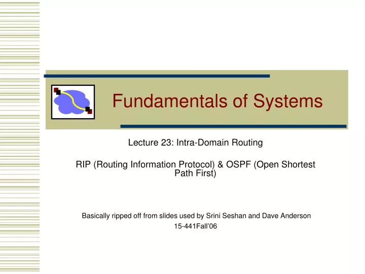
Fundamentals of Systems. Lecture 23: Intra-Domain Routing RIP (Routing Information Protocol) & OSPF (Open Shortest Path First) Basically ripped off from slides used by Srini Seshan and Dave Anderson 15-441Fall’06. Outline. Review/Overview Routing Hierarchy Distance Vector Link State.

E N D
Fundamentals of Systems Lecture 23: Intra-Domain Routing RIP (Routing Information Protocol) & OSPF (Open Shortest Path First) Basically ripped off from slides used by Srini Seshan and Dave Anderson 15-441Fall’06
Outline • Review/Overview • Routing Hierarchy • Distance Vector • Link State Lecture 10: Intra-Domain Routing
Router IP Forwarding • The Story So Far… • IP addresses are structure to reflect Internet structure • IP packet headers carry these addresses • When Packet Arrives at Router • Examine header to determine intended destination • Look up in table to determine next hop in path • Send packet out appropriate port • This/next lecture • How to generate the forwarding table Lecture 10: Intra-Domain Routing
Graph Model • Represent each router as node • Direct link between routers represented by edge • Symmetric links undirected graph • Edge “cost” c(x,y) denotes measure of difficulty of using link • delay, $ cost, or congestion level • Task • Determine least cost path from every node to every other node • Path cost d(x,y) = sum of link costs E C 3 1 F 1 2 6 1 D 3 A 4 B Lecture 10: Intra-Domain Routing
Routes from Node A • Properties • Some set of shortest paths forms tree • Shortest path spanning tree • Solution not unique • E.g., A-E-F-C-D also has cost 7 E C 3 1 F 1 2 6 1 D 3 A 4 B Lecture 10: Intra-Domain Routing
Ways to Compute Shortest Paths • Centralized • Collect graph structure in one place • Use standard graph algorithm • Disseminate routing tables • Link-state • Every node collects complete graph structure • Each computes shortest paths from it • Each generates own routing table • Distance-vector • No one has copy of graph • Nodes construct their own tables iteratively • Each sends information about its table to neighbors Lecture 10: Intra-Domain Routing
Outline • Review/Overview • Routing Hierarchy • Distance Vector • Link State Lecture 10: Intra-Domain Routing
Routing Hierarchies • Flat routing doesn’t scale • Storage Each node cannot be expected to store routes to every destination (or destination network) • Convergence times increase • Communication Total message count increases • Key observation • Need less information with increasing distance to destination • Need lower diameters networks • Solution: area hierarchy Lecture 10: Intra-Domain Routing
Areas • Divide network into areas • Areas can have nested sub-areas • Hierarchically address nodes in a network • Sequentially number top-level areas • Sub-areas of area are labeled relative to that area • Nodes are numbered relative to the smallest containing area Lecture 10: Intra-Domain Routing
Routing Hierarchy Backbone Areas • Partition Network into “Areas” • Within area • Each node has routes to every other node • Outside area • Each node has routes for other top-level areas only • Inter-area packets are routed to nearest appropriate border router • Constraint: no path between two sub-areas of an area can exit that area Area-Border Router Lower-level Areas Lecture 10: Intra-Domain Routing
Area Hierarchy Addressing 1 2 2.2 2.1 1.1 2.2.2 1.2 2.2.1 1.2.1 1.2.2 3 3.2 3.1 Lecture 10: Intra-Domain Routing
Path Sub-optimality • Can result in sub-optimal paths 1 2 2.1 2.2 1.1 2.2.1 1.2 1.2.1 start end 3.2.1 3 3 hop red path vs. 2 hop green path 3.2 3.1 Lecture 10: Intra-Domain Routing
Outline • Review/Overview • Routing Hierarchy • Distance Vector • Link State Lecture 10: Intra-Domain Routing
Distance-Vector Method • Idea • At any time, have cost/next hop of best known path to destination • Use cost when no path known • Initially • Only have entries for directly connected nodes E C 3 1 F 1 2 6 1 D 3 A 4 B Lecture 10: Intra-Domain Routing
Distance-Vector Update z • Update(x,y,z) d c(x,z) + d(z,y) # Cost of path from x to y with first hop z if d < d(x,y) # Found better path return d,z# Updated cost / next hop else return d(x,y), nexthop(x,y) # Existing cost / next hop d(z,y) c(x,z) y x d(x,y) Lecture 10: Intra-Domain Routing
Algorithm • Bellman-Ford algorithm • Repeat For every node x For every neighbor z For every destination y d(x,y) Update(x,y,z) • Until converge Lecture 10: Intra-Domain Routing
Start Optimum 1-hop paths E C 3 1 F 1 2 6 1 D 3 A 4 B Lecture 10: Intra-Domain Routing
Iteration #1 Optimum 2-hop paths E C 3 1 F 1 2 6 1 D 3 A 4 B Lecture 10: Intra-Domain Routing
Iteration #2 Optimum 3-hop paths E C 3 1 F 1 2 6 1 D 3 A 4 B Lecture 10: Intra-Domain Routing
1 4 1 50 X Z Y Distance Vector: Link Cost Changes • Link cost changes: • Node detects local link cost change • Updates distance table • If cost change in least cost path, notify neighbors algorithm terminates “good news travels fast” Lecture 10: Intra-Domain Routing
60 4 1 50 X Z Y Distance Vector: Link Cost Changes • Link cost changes: • Good news travels fast • Bad news travels slow - “count to infinity” problem! algorithm continues on! Lecture 10: Intra-Domain Routing
60 4 1 50 X Z Y Distance Vector: Split Horizon • If Z routes through Y to get to X : • Z does not advertise its route to X back to Y algorithm terminates ? ? ? Lecture 10: Intra-Domain Routing
60 4 1 50 X Z Y Distance Vector: Poison Reverse • If Z routes through Y to get to X : • Z tells Y its (Z’s) distance to X is infinite (so Y won’t route to X via Z) • Eliminates some possible timeouts with split horizon • Will this completely solve count to infinity problem? algorithm terminates Lecture 10: Intra-Domain Routing
1 F C 6 A 1 4 1 B D Poison Reverse Failures • Iterations don’t converge • “Count to infinity” • Solution • Make “infinity” smaller • What is upper bound on maximum path length? Forced Update Forced Update Better Route Forced Update Forced Update • • • Forced Update Lecture 10: Intra-Domain Routing
Routing Information Protocol (RIP) • Earliest IP routing protocol (1982 BSD) • Current standard is version 2 (RFC 1723) • Features • Every link has cost 1 • “Infinity” = 16 • Limits to networks where everything reachable within 15 hops • Sending Updates • Every router listens for updates on UDP port 520 • RIP message can contain entries for up to 25 table entries Lecture 10: Intra-Domain Routing
RIP Updates • Initial • When router first starts, asks for copy of table for every neighbor • Uses it to iteratively generate own table • Periodic • Every 30 seconds, router sends copy of its table to each neighbor • Neighbors use to iteratively update their tables • Triggered • When ever an entry changes, send copy of entry to neighbors • Except for one causing update (split horizon rule) (*NOTE*) • Neighbors use to update their tables • Not immediate, but slight delay to prevent cascading updates Lecture 10: Intra-Domain Routing
RIP Staleness / Oscillation Control • Small Infinity • Count to infinity doesn’t take very long • Timers • Update: 30 seconds (Periodic advertisements • Time-out: 180s (Route is dead if update not heard within this period) • Flush: 120s (Wait after time-out before deleting, during this time advertised as infinity) • Hold-down [Not standard]: 90s, typical (Freeze unreachable route to prevent receiving dated information) • Behavior • When router or link fails, can take minutes to stabilize Lecture 10: Intra-Domain Routing
Outline • Review/Overview • Routing Hierarchy • Distance Vector • Link State Lecture 10: Intra-Domain Routing
Link State Protocol Concept • Every node gets complete copy of graph • Every node “floods” network with data about its outgoing links • Every node computes routes to every other node • Using single-source, shortest-path algorithm • Process performed whenever needed • When connections die / reappear Lecture 10: Intra-Domain Routing
Sending Link States by Flooding • X Wants to Send Information • Sends on all outgoing links • When Node Y Receives Information from Z • Send on all links other than Z X A X A C B D C B D (a) (b) X A X A C B D C B D (c) (d) Lecture 10: Intra-Domain Routing
Dijkstra’s Algorithm • Given • Graph with source node s and edge costs c(u,v) • Determine least cost path from s to every node v • Shortest Path First Algorithm • Traverse graph in order of least cost from source Lecture 10: Intra-Domain Routing
Node Sets Done Already have least cost path to it Horizon: Reachable in 1 hop from node in Done Unseen: Cannot reach directly from node in Done Label d(v) = path cost From s to v Path Keep track of last link in path 2 5 Current Path Costs 0 3 Dijkstra’s Algorithm: Concept E C 3 1 F 2 2 6 1 Source Node D 3 A 3 B Done Unseen Horizon Lecture 10: Intra-Domain Routing
Current Path Costs 0 Dijkstra’s Algorithm: Initially • No nodes done • Source in horizon E C 3 1 F 2 2 6 1 Source Node D 3 A 3 B Horizon Done Unseen Lecture 10: Intra-Domain Routing
2 6 Current Path Costs 0 3 Dijkstra’s Algorithm: Initially • d(v) to node A shown in red • Only consider links from done nodes E C 3 1 F 2 2 6 1 Source Node D 3 A 3 B Done Unseen Horizon Lecture 10: Intra-Domain Routing
Dijkstra’s Algorithm • Select node v in horizon with minimum d(v) • Add link used to add node to shortest path tree • Update d(v) information E C 2 3 5 6 1 Current Path Costs F 2 2 6 1 Source Node 0 D 3 3 A 3 B Done Unseen Horizon Lecture 10: Intra-Domain Routing
2 5 Current Path Costs 0 3 Dijkstra’s Algorithm • Repeat… Horizon E C 3 1 F 2 2 6 1 Source Node D 3 A 3 B Done Unseen Lecture 10: Intra-Domain Routing
2 4 Current Path Costs 0 6 3 Dijkstra’s Algorithm Unseen • Update d(v) values • Can cause addition of new nodes to horizon E C 3 1 F 2 2 6 1 Source Node D 3 A 3 B Horizon Done Lecture 10: Intra-Domain Routing
5 2 4 0 6 3 Dijkstra’s Algorithm • Final tree shown in green E C 3 1 F 2 2 6 1 Source Node D 3 A 3 B Lecture 10: Intra-Domain Routing
Link State Characteristics • With consistent LSDBs*, all nodes compute consistent loop-free paths • Can still have transient loops B 1 1 X 3 A C 5 2 D Packet from CA may loop around BDC if B knows about failure and C & D do not • Link State Data Base Lecture 10: Intra-Domain Routing
OSPF Routing Protocol • Open • Open standard created by IETF • Shortest-path first • Another name for Dijkstra’s algorithm • More prevalent than RIP • Uses IP directly, not UDP • Multicast to reduce network load Lecture 10: Intra-Domain Routing
OSPF Reliable Flooding • Transmit link state advertisements • Originating router • Typically, minimum IP address for router • Link ID • ID of router at other end of link • Metric • Cost of link [Unlike RIP can be anything] • Link-state age • Incremented each second • Packet expires when reaches 3600 • Sequence number • Incremented each time sending new link information Lecture 10: Intra-Domain Routing
OSPF Flooding Operation • Node X Receives LSA from Node Y • With Sequence Number q • Looks for entry with same origin/link ID • Cases • No entry present • Add entry, propagate to all neighbors other than Y • Entry present with sequence number p < q • Update entry, propagate to all neighbors other than Y • Entry present with sequence number p > q • Send entry back to Y • To tell Y that it has out-of-date information • Entry present with sequence number p = q • Ignore it Lecture 10: Intra-Domain Routing
Flooding Issues • When should it be performed • Periodically • When status of link changes • Detected by connected node • What happens when router goes down & back up • Sequence number reset to 0 • Other routers may have entries with higher sequence numbers • Router will send out LSAs with number 0 • Will get back LSAs with last valid sequence number p • Router sets sequence number to p+1 & resends Lecture 10: Intra-Domain Routing
Adoption of OSPF • RIP viewed as outmoded • Good when networks small and routers had limited memory & computational power • OSPF Advantages • Fast convergence when configuration changes Lecture 10: Intra-Domain Routing
Message complexity LS: with n nodes, E links, O(nE) messages DV: exchange between neighbors only Speed of Convergence LS: Complex computation But…can forward before computation may have oscillations DV: convergence time varies may be routing loops count-to-infinity problem (faster with triggered updates) Space requirements: LS maintains entire topology DV maintains only neighbor state Comparison of LS and DV Algorithms Lecture 10: Intra-Domain Routing
Comparison of LS and DV Algorithms • Robustness: what happens if router malfunctions? • LS: • node can advertise incorrect link cost • each node computes only its own table • DV: • DV node can advertise incorrect path cost • each node’s table used by others • errors propagate thru network • Other tradeoffs • Making LSP flood reliable Lecture 10: Intra-Domain Routing
Next Lecture: BGP, DNS • How to connect together different ISPs • The Domain Name System Lecture 10: Intra-Domain Routing