Download
1 / 17
170 likes | 303 Views
Introduction to Heat Transfer. Finite Difference Methods Or Computational Calculus. The Microwave Oven. Consider the problem of heating your lunch in a microwave oven Given a known heating rate, calculate the time and temperature of your lunch

E N D
Introduction to Heat Transfer Finite Difference Methods Or Computational Calculus
The Microwave Oven • Consider the problem of heating your lunch in a microwave oven • Given a known heating rate, calculate the time and temperature of your lunch Is this answer helpful? Does it represent the real world? Take a bite – why is the center cold (frozen) and edges burning hot? Treating the problem as uniform temperature does not work. This problem needs the tools of calculus.
Computational Calculus • Break up space into small pieces (cells or zones) • Solve simple equations on each cell • As the cell size goes to zero, the solution approaches the correct values We will use the Introduction to Finite Difference Methods for Numerical Fluid Dynamics by Scannapieco and Harlow to see how to write a computational heat transfer code.
1D Heat FlowDomain Discretization • We will read through Chapter II, pages 6-17 and construct the numerical model given there • Page 6 • Note breaking up rod into zones or elements. Each zone will be an element in an array that we declare • Note definition of finite difference *Discretization is just a fancy way of saying break into small zones (literally make discrete)
1D Heat FlowDefinitions and Fick’s Law • Page 7 • Definition of flux and conservation • Flux is the motion of something from one cell to another • Conservation is keeping the same total amount of things like mass and energy. This keeps simulations from being non-physical. • Page 8 • Note the equation for an individual cell (zone) • Fick’s Law is what you should see in high school physics and should be intuitive
1D Heat FlowComputational Model • Bottom page 8 and top page 9 • The full model is shown with jbar cells • Temperatures are defined at cell centers (j) • Fluxes occur at interfaces between cells (j-½,j+½) • Boundary cells are added at each end for simplicity in implementing boundary conditions (array size will be 0 to j+1 • Bottom page 9, top 10 • Note the equations – simple, but lets check them • These define energy for this problem – we will want to conserve this energy
1D Heat FlowTime Discretization • Page 10 – middle top • In this section, the time domain is broken up into small pieces for the computation. This is similar to what was done with the space dimension and also uses calculus concepts of breaking things into pieces. • Note the superscript represents time, not a power • The time step, dt, must be small enough that all of the heat does not flux out of any cell (a little more complicated than this, but it gets the basic concept).
1D Heat FlowEquation for a single zone • Bottom page 10 to top page 11 • Refer back to the diagram for a single cell or a single cell and its two neighbors • We do a “black box” solution where we don’t worry about what is going on inside a cell and just calculate what is crossing the boundaries • Write the equations for these fluxes and insert into Fick’s law. • Rearrange so that Tn+1 is on the left (actually dT or the change in temperature for the cell)
1D Heat FlowThe Calculus • Section C • We will skip this section and leave it for you to read through. It uses calculus to come up with the same equation • But we will take a quick look at equations II-18 and II-19 and replace ∂T with Tn+1-Tn, ∂x with dx and ∂t with dt. Move dt over to the right and it becomes the same as II-12. II-19 is Fick’s Law as written in calculus
1D Heat FlowComputational Implementation • Declare an array size j+1 • Set initial temperature value • Set boundary conditions on ghost zones (0 and j+1) • Compute new temperatures as shown on pg 16. Note use of T and Tnew and discussion. • Loop back up to setting boundary condition and repeat until we reach time of interest • Print out temperature array
Sample Implementations • Class will write a code in Python or C and see if they can get the results shown on pgs 17-19. Note scales are 0-50 for x axis and 0-400 for y axis. • Advanced • Data can be imported into Excel or other plotting programs for a better graph • Real-time visualization routines can be used to view the simulation during the calculation
C Code #include <stdio.h> intmain(intargc, char *argv[]){ int j, jbar=50; // Problem settings double dx=1.0, dt=0.1, sig=1.0, endtime=10.0, time=0.0, TL=400.0, TR=0.0; double T[jbar+2], Tnew[jbar+2]; // Declare arrays for ( j = 0; j <=jbar+1; j++ ) { T[j] = 0.0;} // Initialize to zero temperature while ( time <= endtime ) { // Loop until time of interest T[0] = 2.0*TL – T[1] T[jbar+1] = 2.0*TR-T[jbar]; // Set boundary conditions for (j=1; j<= jbar; j++) { Tnew[j] = T[j] + sig*dt*(T[j+1]+T[j-1]-2.0*T[j])/dx/dx; // Fick’s Law } for (j=1; j<= jbar; j++) { T[j]=Tnew[j]; } // Copy data back to original array time += dt; // Advance time } for ( j=1; j<=jbar; j++ ) { printf(“x %11.6lf T %11.6lf\n”,((double)(j-1)+0.5)*dx,T[j]); // print results } }
C++ Code (no objects) #include <iostream> #include <vector> using namespace std; intmain(intargc, char *argv[]){ intjbar=50; // Problem settings double dx=1.0, dt=0.1, sig=1.0, endtime=10.0, time=0.0, TL=400.0, TR=0.0; vector<double> T[jbar+2], Tnew[jbar+2]; // Declare arrays for ( j = 0; j <=jbar+1; j++ ) { T[j] = 0.0;} // Initialize to zero temperature while ( time <= endtime ) { // Loop until time of interest T[0] = 2.0*TL – T[1] T[jbar+1] = 2.0*TR-T[jbar]; // Set boundary conditions for (j=1; j<= jbar; j++) { Tnew[j] = T[j] + sig*dt*(T[j+1]+T[j-1]-2.0*T[j])/dx/dx; // Fick’s Law } for (j=1; j<= jbar; j++) { T[j]=Tnew[j]; } // Copy data back to original array time += dt; // Advance time } for ( j=1; j<=jbar; j++ ) { cout << "x " << ((double)(j-1)+0.5)*dx << " T " << T[j] << "\n"; } }
Fortran90 code program heat integer :: j integer, parameter :: jbar=50 ! Problem settings double precision :: dx=dble(1.0), dt=dble(0.1), sig=dble(1.0), endtime=dble(10.0), time=dble(0.0) double precision :: TL = dble(400.0), TR = dble(0.0) double precision :: T(0:jbar+1), Tnew(0:jbar+1) ! Declare arrays T(:) = dble(0.0) ! Initialization do if ( time > endtime ) exit T(0) = dble(2.0)*TL - T(1) ! Boundary conditions T(jbar+1) = dble(2.0)*TR - T(jbar) do j=1,jbar Tnew(j) = T(j) + sig*dt*(T(j+1)+T(j-1)-dble(2.0)*T(j))/dx/dx ! Fick’s law end do T(1:jbar) = Tnew(1:jbar) ! Copy data back to original array time = time + dt ! Advance time end do do j=1,jbar write(*,'(2(a,f11.6))') "x ",(dble(j-1)+dble(0.5))*dx," T ", T(j) ! Print results end do end program
Python Code bar = 50 # Problem setting dx=1.0; dt=0.1; sig=1.0; endtime=10.0; time=0.0; TL=400.0; TR=0.0 T = [ 0.00 for j in range(0, jbar + 2) ] # Declare and initialize arrays Tnew = T[:] j = jbar while time <= endtime: T[0] = 2.0*TL - T[1] # Boundary conditions T[jbar+1] = 2.0*TR-T[jbar] for j in range(1, jbar+1): Tnew[j] = T[j] + sig*dt*(T[j+1]+T[j-1]-2.0*T[j])/dx/dx; # Fick’s Law for j in range(1, jbar): T[j] = Tnew[j] # Copy data to original array time += dt # Advance time for j in range(1, jbar+1): print "x %11.6lf T %11.6lf" % ( ((j-1)+0.5)*dx, T[j] ) # Print results
Results from 1st case x 0.500000 T 364.403880 x 1.500000 T 294.969983 x 2.500000 T 230.553041 x 3.500000 T 173.699977 x 4.500000 T 125.958989 x 5.500000 T 87.809097 x 6.500000 T 58.791526 x 7.500000 T 37.777208 x 8.500000 T 23.283011 x 9.500000 T 13.758309 x 10.500000 T 7.792707 x 11.500000 T 4.229989 x 12.500000 T 2.200338 x 13.500000 T 1.096845 x 14.500000 T 0.524013 x 15.500000 T 0.239960 x 16.500000 T 0.105345 x 17.500000 T 0.044346 x 18.500000 T 0.017905 x 19.500000 T 0.006936 x 20.500000 T 0.002578 x 21.500000 T 0.000920 x 22.500000 T 0.000315 x 23.500000 T 0.000104 x 24.500000 T 0.000033 x 25.500000 T 0.000010 x 26.500000 T 0.000003 x 27.500000 T 0.000001 x 28.500000 T 0.000000 x 29.500000 T 0.000000 x 30.500000 T 0.000000 x 31.500000 T 0.000000 x 32.500000 T 0.000000 x 33.500000 T 0.000000 x 34.500000 T 0.000000 x 35.500000 T 0.000000 x 36.500000 T 0.000000 x 37.500000 T 0.000000 x 38.500000 T 0.000000 x 39.500000 T 0.000000 x 40.500000 T 0.000000 x 41.500000 T 0.000000 x 42.500000 T 0.000000 x 43.500000 T 0.000000 x 44.500000 T 0.000000 x 45.500000 T 0.000000 x 46.500000 T 0.000000 x 47.500000 T 0.000000 x 48.500000 T 0.000000 x 49.500000 T 0.000000
Further Investigations • Time step stability is discussed starting on pg. 20. You can try this with the class model • Fluid dynamic models of various types are discussed in later chapters. • Simple turbulence models are studied. And now we can study the microwave problem – does it help to put more heat at the surface (Increase TL)? What is the fastest way to heat the food? the most energy efficient? the most even heating?