Download
1 / 122
1.23k likes | 1.26k Views
Microwave Interaction with Atmospheric Constituents. Chris Allen (callen@eecs.ku.edu) Course website URL people.eecs.ku.edu/~callen/823/EECS823.htm. Outline. Physical properties of the atmosphere Absorption and emission by gases Water vapor absorption Oxygen absorption

E N D
Microwave Interaction with Atmospheric Constituents • Chris Allen (callen@eecs.ku.edu) • Course website URL people.eecs.ku.edu/~callen/823/EECS823.htm
Outline • Physical properties of the atmosphere • Absorption and emission by gases • Water vapor absorption • Oxygen absorption • Extraterrestrial sources • Extinction and emission by clouds and precipitation • Single particle effects • Mie scattering • Rayleigh approximation • Scattering and absorption by hydrometeors • Volume scattering and absorption coefficients • Extinction and backscattering • Clouds, fog, and haze • Rain • Snow • Emission by clouds and rain
Physical properties of the atmosphere • The gaseous composition, and variations of temperature, pressure, density, and water-vapor density with altitude are fundamental characteristics of the Earth’s atmosphere. • Atmospheric scientists have developed standard models for the atmosphere that are useful for RF and microwave models. • These models are representative and variations with latitude, season, and region may be expected.
Temperature, density, pressure profile • Atmospheric density, pressure, and water-vapor density decrease exponentially with altitude. • The atmosphere is subdivided based on thermal profile and thermal gradients (dT/dz) where z is altitude. Troposphere surface to about 10 km dT/dz ~ -6.5 C km-1 Stratosphere upper boundary ~ 47 kmdT/dz ~ 2.8 C km-1 above ~ 32 km Mesosphere upper boundary 80 to 90 kmdT/dz ~ -3.5 C km-1 above ~ 60 km
Temperature model • Only the lowermost 30 km of the atmosphere significantly affects the microwave and RF signals due to the exponential decrease of density with altitude. • For this region a simple piece-wise linear model for the atmospheric temperature T(z) vs. altitude may be used. • Here T(z) is expressed in K, T0 is the sea-level temperature and T(11) is the atmospheric temperature at 11 km. For the 1962 U.S. Standard Atmosphere, the thermal gradient term a is -6.5 C km-1 and T0 = 288.15 K.
Density and pressure models • For the lowermost 30 km of the atmosphere a model that predicts the variation of dry air density airwith altitude is • where air has units of kg m-3, z is the altitude in km, H2 is 7.3 km. • Assuming air to be an ideal gas we can apply the ideal gas law to predict the pressure P at any altitude (up to 30 km above sea level) using • Alternatively pressure can be found using • where H3 = 7.7 km and Po = 1013.25 mbar
Water-vapor density model • The water-vapor content of the atmosphere is weather dependent and largely temperature driven. • The sea-level water vapor density can vary from 0.01 g m-3 in cold dry climates to 30 g m-3 in warm, humid climates. • An average value for mid-latitude regions is 7.72 g m-3. • Using this value as the surface value at sea-level, we can use the following model to predict the water-vapor density v at any altitude using • where v has units of g m-3, 0 is 7.72 g m-3, and H4 is 2 km.
Absorption and emission by gases • Molecular absorption (and emission) of electromagnetic energy may involve three types of energy states • where Ee = electronic energy Ev = vibrational energy Er = rotational energy • Of the various gases and vapors in the Earth’s atmosphere, only oxygen and water vapor have significant absorption bands in the microwave spectrum. • Oxygen’s magnetic moment enables rotational energy states around 60 GHz and 118.8 GHz. • Water vapor’s electric dipole enables rotational energy states at 22.2 GHz, 183.3 GHz, and several frequencies above 300 GHz.
Spectral line shape • For a molecule in isolation the absorption and emission energy levels are very precise and produce well defined spectral lines. Energy exchanges and interactions in the form of collisions result in a spectral line broadening. One mechanism that produces spectral line broadening is termed pressure broadening as it results from collisions between molecules.
Absorption spectrum model • The absorption spectrum for transactions between a pair of energy states may be written as • where a = power absorption coefficient, Np m-1 f = frequency, Hz flm = molecular resonance frequency for transitions between energy states El and Em, Hz c = speed of light, 3 108 m s-1 Slm= line strength of the lm line, Hz F = line-shape function, Hz-1 • The line strength Slm of the lm line depend on the number of absorbing gas molecules per unit volume, gas temperature, and molecular parameters.
Line-shape function • There are several different line-shape functions, F, used to describe the shape of the absorption spectrum with respect to the resonance frequency, flm. • The Lorentzian function, FL, is the simplest • here • = linewidth parameter, Hz The Van Vleck and Weisskopf function, FVW, takes into account atmospheric pressures
Line-shape function • The Gross function, FG, was developed using a different approach and shows better agreement with measured data further from the resonance frequency.
Water-vapor absorption • Absorption due to water vapor can be modeled using • For each water-vapor absorption line the line strength is • where Slm0 = constant characteristic of the lm transition flm = the resonance frequency v = water-vapor density El = lower energy state’s energy level k = Boltzmann’s constant (1.38 10-23 J K-1) T = thermodynamic temperature (K) • Thus (f, flm) expressed in dB km-1 is
Water-vapor absorption • Water vapor has resonant frequencies at 22.235 GHz, 183.31 GHz, 323 GHz, 325.1538 GHz, 380.1968 GHz, 390 GHz, 436 GHz, 438 GHz, 442 GHz, … • For frequencies below 100 GHz we may consider the water-vapor absorption coefficient to be composed of two factors • Where (f, 22) = absorption due to 22.235-GHz resonance r(f) = residual term representing absorption due to all higher- frequency water-vapor absorption lines
Water-vapor absorption • Using data for the 22.235-GHz resonance we get • where the linewidth parameter 1 is • f and 1 are expressed in GHz, T is in K, v is in g m-3, andP is in millibars. • The residual absorption term is • Therefore the total water vapor absorption below 100 GHz is
Oxygen absorption • Molecular oxygen has numerous absorption lines between 50 and 70 GHz (known as the 60-GHz complex) as well as a line at 118.75 GHz. • Around 60 GHz there are 39 discrete resonant frequencies that blend together due to pressure broadening at the lower altitudes. • Complex models are available that predict the oxygen absorption coefficient throughout the microwave spectrum. • Resonant frequencies (GHz) in the 60-GHz complex: 49.9618, 50.4736, 50.9873, 51.5030, 52.0212, 52.5422, 53.0668, 53.5957, 54.1300, 54.6711, 55.2214, 55.7838, 56.2648, 56.3634, 56.9682, 57.6125, 58.3239, 58.4466, 59.1642, 59.5910, 60.3061, 60.4348, 61.1506, 61.8002, 62.4863, 62.4112, 62.9980, 63.5685, 64.1278, 64.6789, 65.2241, 65.7647, 66.3020, 66.8367, 67.3964, 67.9007, 68.4308, 68.9601, 69.4887
Oxygen absorption • For frequencies below 45 GHz a low-frequency approximation model may be used that combines the effects of all of the resonance lines in the 60-GHz complex with a single resonance at 60 GHz, and that neglects the effect of the 118.75-GHz resonance. • where f is in GHz, f0 = 60 GHz, and
Total atmospheric gaseous absorption • As water vapor and oxygen are the dominant sources for atmospheric absorption (and emission), the total gaseous absorption coefficient is the sum of these two components
Total atmospheric gaseous absorption • Non-zenith optical thickness can be approximated as • for 70°.
Atmospheric gaseous emission • We know that for a non-scattering gaseous atmosphere • where • An upward-looking radiometer would receive the down-welling radiation, TDN, plus a small energy component from cosmic and galactic radiation sources. • where • TCOS and TGAL are the cosmic and galactic brightness temperatures, and TEXTRA is the extraterrestrial brightness temperature.
Extraterrestrial sources • TCOS is independent of frequency and direction. • TGAL is both frequency and direction dependent. • Frequency dependenceDepending on the specific region of the galaxy, • Above 5 GHz, TGAL« TDN and TGAL may be neglected. • Below 1 GHz TGAL may not be ignored.TGAL plus man-made emissions limit the usefulness of Earth observations below 1 GHz. • Direction dependenceTGAL(max) in the direction of the galactic center while TGAL(min) is the direction of the galactic pole.
Extraterrestrial sources • The galactic center is located in the constellation Sagittarius. Radiation from this location is associated with the complex astronomical radio source Sagittarius A, believed to be a supermassive black hole.
Effects of the sun • The sun’s brightness temperature TSUN is frequency dependent as well as dependent on the “state” of the sun. • For the “quiet” sun (no significant sunspots or flares) TSUN decreases with increasing frequency. • At 100 MHz, TSUN is about 106 K, while at 10 GHz it is 104 K, and above 30 GHz TSUN is 6000 K. • When sunspots and flares are present, TSUN can increase by orders of magnitude. • Jupiter, a star wannabe, also emits significant energy though it is smaller than the active sun by at least two orders of magnitude.
Other radio stars • Taken from: Preston, GW; “The Theory of Stellar Radar,” Rand Corp. Memorandum RM-3167-PR, May 1962. • The radio stars (Cassiopeia A, Cygnus A, Centaurus A, Virgo, etc.) are astounding sources of RF energy, not only because of their great strength, but also because of their remarkable energy spectra. • These spectra reach their maxima at about 10 m wavelength (30 MHz in frequency) and fall off rather sharply at higher frequencies (~ 10 dB/decade). • The flux density from Cassiopeia exceeds the solar flux at longer wavelengths. • Compared to Cassiopeia, Cygnus is 2 dB weaker, Centaurus is 8 dB weaker, and Virgo is 10 dB weaker.
Extinction and emission by clouds and precipitation • Electromagnetic interaction with individual spherical particles • A spherical particle with a radius r is illuminated by an electromagnetic plane wave with power density Si [W m-2], a portion of which is absorbed, Pa. • The absorption cross-section, Qa is • The absorption efficiency factor, a, is the ratio of Qa to the geometrical cross-section, A, is
Electromagnetic interaction with individual spherical particles • If the incident wave were traveling along the +z axis, and Ss(, ) is the power density radiation scattered in the (, ) direction at distance R, then the total power scattered by the particle is • The scattering cross section, Qs and the scattering efficiency factor, s are • Thus Pa + Ps represent the total power removed from the incident wave and the extinction cross sectionQe and extinction efficiency e are
Electromagnetic interaction with individual spherical particles • For monostatic radar applications, the radar backscattering cross-sectionb is of interest and this is that portion of Ss(, ) directed back toward the radiation source, i.e.,Ss( = ) or Ss(). • Note:Incident wave travels along the +z axis,so = corresponds to backscatter direction.Also, when = , has no significance. • b is defined as • or
Mie scattering • Gustov Mie, in 1908, developed the complete solution for the scattering and absorption of a dielectric sphere of arbitrary radius, r, composed of a homogeneous, isotropic and optically linear material irradiated by an infinitely extending plane wave. • Key terms are the Mie particle size parameter and the refractive index n (refractive contrast?) • where ′rb = real part of relative dielectric constant of background medium cb = complex dielectric constant of background medium (F m-1) cp = complex dielectric constant of particle medium (F m-1) 0 = free-space wavelength (m) b = wavelength in background medium (m)
Mie scattering • Numerical solutions for spheres of various composition. • “optical” limit e = 2 for » 1
Mie scattering • Strongly conducting sphere • For << 1, s << a
Mie scattering • Weakly absorbing sphere • Again, for «1, s« aso e a • Also, as , a 1and s 1 if 0 < n″« 1
Backscattering efficiency, b • Mie’s solution also predicts the backscattering efficiency, b, for a spherical particle • “optical” limit b = 1 for » 1
Rayleigh approximation • For particles much smaller than the incident wave’s wavelength, i.e., |n | « 1, the Mie solution can be approximated with simple expressions known as the Rayleigh approximations. • For |n | < 0.5 (Rayleigh region) • where • and • Unless the partical is weakly absorbing (i.e., n″« n′)such thatIm{-K} « |K|2, Qa» Qs since Qs varies as 6 and Qa varies as 3.
Rayleigh approximation • Therefore the scattering cross section increases quite rapidly with particle radius and with increasing frequency. • ExampleFor held constant, a 12% increase in radius r (a 40% volume increase) doubles the scattering cross section. • For a constant radius r, an octave increase in frequency (factor of 2) results in a 16-fold increase (12 dB) in the scattering cross section. • and • so
Rayleigh backscattering • Again, for the Rayleigh region (|n | < 0.5), a simplified expression for the backscattering efficiency is found, Rayleigh’s backscattering law • or • And as was the case for the scattering cross section, • Therefore in the Rayleigh region, the backscattering cross section is very sensitive to particle size relative to wavelength.
Rayleigh backscattering • For large |n|, |K| 1 yielding • However for the case of |n| = (perfect conductor) which violates the Rayleigh condition (|n | < 0.5) for finite particle sizes, the backscattering cross section can be found for || «1 using Mie’s solution • or
Scattering and absorption by hydrometeors • Now we consider the interaction of RF and microwave waves with hydrometeors (i.e., precipitation product, such as rain, snow, hail, fog, or clouds, formed from the condensation of water vapor in the atmosphere). • Electromagnetic scattering and absorption of a spherical particle depend on three parameters: wavelength, particle’s complex refractive index, n particle radius, r • This requires an understanding of the dielectric properties of liquid water and ice.
Pure water • The Debye equation describes the frequency dependence of the dielectric constant of pure water, w • where w0 = static relative dielectric constant of pure water, dimensionless w = high-frequency (or optical) limit of w, dimensionless w = relaxation time of pure water, s f = electromagnetic frequency, Hz • Algebraic manipulation yields
Pure water • While w is apparently temperature independent, temperature affects w0 and w causing ′w and ″w to be dependent on temperature, T. • The relaxation time for pure water is • where T is expressed in C. • The corresponding relaxation frequency fw0 of pure water is • which varies from 9 GHz at 0 C to 17 GHz at 20 C. • The temperature-dependent static dielectric of water is
Pure water • Relative dielectric constant, real part, r′ vs. imaginary part, r″
Pure water • To apply the solutions from Mie or Rayleigh requires the complex refractive index. • where rc is the complex relative dielectric constant
Pure water • Refractive index, real part, n′
Pure water • Refractive index, imaginary part, n″
Pure water • Refractive index, magnitude |n|
Sea water • Saline water is water containing dissolved salts. • The salinity, S, is the total salt mass in grams dissolved in 1 kg of water and is typically expressed in parts per thousand (‰) on a gravimetric (weight) basis. • The average sea-water salinity, Ssw, is 32.54 ‰ • The following expressions for the real and imaginary parts of the relative dielectric constant of saline water are valid over salinity range of 4 to 35 ‰ and the temperature range from 0 to 40 C. • where sw is the relaxation time of saline water, s i is the ionic conductivity of the aqueous soluiton, S m-1 0 is the free-space permittivity, 8.854 10-12 F m-1
Sea water • The high-frequency (or optical) limit of sw is independent of salinity. • The static relative dielectric constant of saline water depends on salinity (‰) and temperature (C). • where