Download
1 / 73
730 likes | 734 Views
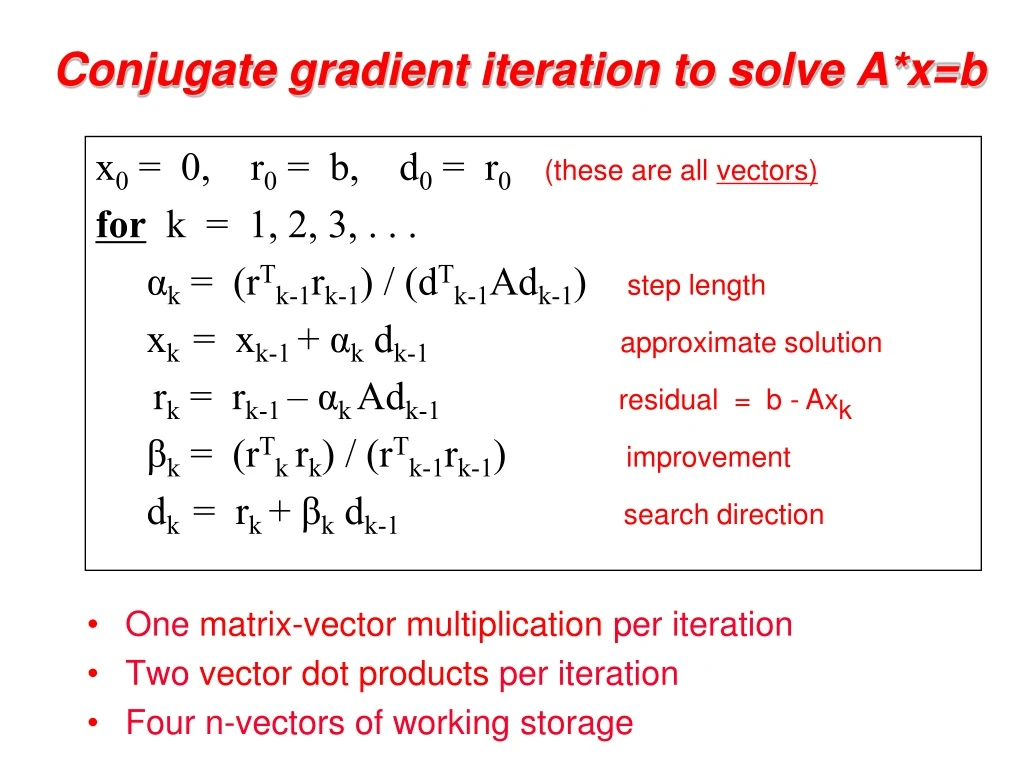
This algorithm uses the Conjugate Gradient Iteration method to solve the equation A*x=b. It iteratively updates the solution vector x and computes the residual vector r. The algorithm employs matrix-vector multiplication, vector dot products, and working storage vectors.

E N D
Conjugate gradient iteration to solve A*x=b x0 = 0, r0 = b, d0 = r0 (these are all vectors) for k = 1, 2, 3, . . . αk = (rTk-1rk-1) / (dTk-1Adk-1) step length xk= xk-1 + αk dk-1 approximate solution rk = rk-1 – αk Adk-1 residual = b - Axk βk = (rTkrk) / (rTk-1rk-1) improvement dk= rk+ βk dk-1 search direction • One matrix-vector multiplication per iteration • Two vector dot products per iteration • Four n-vectors of working storage
Vector and matrix primitives for CG • DAXPY: v = α*v + β*w (vectors v, w; scalars α, β) • Broadcast the scalars α and β, then independent * and + • comm volume = 2p, span = log n • DDOT: α = vT*w = Sjv[j]*w[j](vectors v, w; scalar α) • Independent *, then + reduction • comm volume = p, span = log n • Matvec: v = A*w (matrix A, vectors v, w) • The hard part • But all you need is a subroutine to compute v from w • Sometimes you don’t need to store A (e.g. temperature problem) • Usually you do need to store A, but it’s sparse ...
Broadcast and reduction • Broadcast of 1 value to p processors in log p time • Reduction of p values to 1 in log p time • Takes advantage of associativity in +, *, min, max, etc. α Broadcast 1 3 1 0 4 -6 3 2 Add-reduction 8
P0 P1 P2 P3 x P0 P1 P2 P3 y Parallel sparse matrix-vector product • Lay out matrix and vectors by rows • y(i) = sum(A(i,j)*x(j)) • Only compute terms with A(i,j) ≠ 0 • Algorithm Each processor i: Broadcast x(i) Compute y(i) = A(i,:)*x • Optimizations • Only send each proc the parts of x it needs, to reduce comm • Reorder matrix for better locality by graph partitioning • Worry about balancing number of nonzeros / processor, if rows have very different nonzero counts
Data structure for sparse matrix A (stored by rows) • Full matrix: • 2-dimensional array of real or complex numbers • (nrows*ncols) memory • Sparse matrix: • compressed row storage • about (2*nzs + nrows) memory
Distributed-memory sparse matrix data structure Matrix A Processor 0’s slice P0 P1 • Each processor stores: • # of local nonzeros • range of local rows • nonzeros in CSR form P2 Pn
Graphs and Sparse Matrices • Sparse matrix is a representation of a (sparse) graph 1 2 3 4 5 6 1 1 1 2 1 1 1 3 1 11 4 1 1 5 1 1 6 1 1 3 2 4 1 5 6 • Matrix entries are edge weights • Number of nonzeros per row is the vertex degree • Edges represent data dependencies in matrix-vector multiplication
CS 240A: Graph and hypergraph partitioning • Motivation and definitions • Motivation from parallel computing • Theory of graph separators • Heuristics for graph partitioning • Iterative swapping • Spectral • Geometric • Multilevel • Beyond graphs • Shortcomings of the graph partitioning model • Hypergraph models of communication in MatVec • Parallel methods for partitioning hypergraphs
Distributed-memory sparse matrix data structure Matrix A Processor 0’s slice P0 P1 Each processor stores: • # of local nonzeros • range of local rows • nonzeros in CSR form P2 Pn
2D Layout for Sparse Matrices & Vectors Matrix/vector distributions, interleaved on each other. Default distribution in Combinatorial BLAS. Scalable with increasing number of processes 5 8 - 2D matrix layout wins over 1D with large core counts and with limited bandwidth/compute - 2D vector layout sometimes important for load balance
QuadMat shared-memory data structure subdivide by dimension on power of 2 indices m rows Blocks store enough matrix elements for meaningful computation; denser parts of matrix have more blocks. n columns
CS 240A: Graph and hypergraph partitioning • Motivation and definitions • Motivation from parallel computing • Theory of graph separators • Heuristics for graph partitioning • Iterative swapping • Spectral • Geometric • Multilevel • Beyond graphs • Shortcomings of the graph partitioning model • Hypergraph models of communication in MatVec • Parallel methods for partitioning hypergraphs
CS 240A: Graph and hypergraph partitioning • Motivation and definitions • Motivation from parallel computing • Theory of graph separators • Heuristics for graph partitioning • Iterative swapping • Spectral • Geometric • Multilevel • Beyond graphs • Shortcomings of the graph partitioning model • Hypergraph models of communication in MatVec • Parallel methods for partitioning hypergraphs
2 (2) 1 3 (1) 4 1 (2) 2 4 (3) 3 1 2 2 5 (1) 8 (1) 1 6 5 6 (2) 7 (3) Definition of Graph Partitioning • Given a graph G = (N, E, WN, WE) • N = nodes (or vertices), • E = edges • WN = node weights • WE = edge weights • Often nodes are tasks, edges are communication, weights are costs • Choose a partition N = N1 U N2 U … U NP such that • Total weight of nodes in each part is “about the same” • Total weight of edges connecting nodes in different parts is small • Balance the work load, while minimizing communication • Special case of N = N1 U N2: Graph Bisection
Applications • Telephone network design • Original application, algorithm due to Kernighan • Load Balancing while Minimizing Communication • Sparse Matrix times Vector Multiplication • Solving PDEs • N = {1,…,n}, (j,k) in E if A(j,k) nonzero, • WN(j) = #nonzeros in row j, WE(j,k) = 1 • VLSI Layout • N = {units on chip}, E = {wires}, WE(j,k) = wire length • Sparse Gaussian Elimination • Used to reorder rows and columns to increase parallelism, and to decrease “fill-in” • Data mining and clustering • Physical Mapping of DNA
Partitioning by Repeated Bisection • To partition into 2k parts, bisect graph recursively k times
Separators in theory • If G is a planar graph with n vertices, there exists a set of at most sqrt(6n) vertices whose removal leaves no connected component with more than 2n/3 vertices. (“Planar graphs have sqrt(n)-separators.”) • “Well-shaped” finite element meshes in 3 dimensions have n2/3 - separators. • Also some others – trees, graphs of bounded genus, chordal graphs, bounded-excluded-minor graphs, … • Mostly these theorems come with efficient algorithms, but they aren’t used much. • “Random graphs” don’t have good separators. • e.g. Erdos-Renyi random graphs have only n - separators.
CS 240A: Graph and hypergraph partitioning • Motivation and definitions • Motivation from parallel computing • Theory of graph separators • Heuristics for graph partitioning • Iterative swapping • Spectral • Geometric • Multilevel • Beyond graphs • Shortcomings of the graph partitioning model • Hypergraph models of communication in MatVec • Parallel methods for partitioning hypergraphs
Separators in practice • Graph partitioning heuristics have been an active research area for many years, often motivated by partitioning for parallel computation. • Some techniques: • Iterative-swapping (Kernighan-Lin, Fiduccia-Matheysses) • Spectral partitioning (uses eigenvectors of Laplacian matrix of graph) • Geometric partitioning (for meshes with specified vertex coordinates) • Breadth-first search (fast but dated) • Many popular modern codes (e.g. Metis, Chaco, Zoltan) use multilevel iterative swapping
Iterative swapping: Kernighan/Lin, Fiduccia/Mattheyses • Take a initial partition and iteratively improve it • Kernighan/Lin (1970), cost = O(|N|3) but simple • Fiduccia/Mattheyses (1982), cost = O(|E|) but more complicated • Start with a weighted graph and a partition A U B, where |A| = |B| • T = cost(A,B) = S {weight(e): e connects nodes in A and B} • Find subsets X of A and Y of B with |X| = |Y| • Swapping X and Y should decrease cost: • newA = A - X U Y and newB = B - Y U X • newT = cost(newA , newB) < cost(A,B) • Compute newT efficiently for many possible X and Y, (not time to do all possible), then choose smallest
Simplified Fiduccia-Mattheyses: Example (1) 1 0 a b Red nodes are in Part1; black nodes are in Part2. The initial partition into two parts is arbitrary. In this case it cuts 8 edges. The initial node gains are shown in red. -1 1 0 2 c d f e g h 0 3 Nodes tentatively moved (and cut size after each pair): none (8);
Simplified Fiduccia-Mattheyses: Example (2) 1 0 a b The node in Part1 with largest gain is g. We tentatively move it to Part2 and recompute the gains of its neighbors. Tentatively moved nodes are hollow circles. After a node is tentatively moved its gain doesn’t matter any more. -3 1 -2 2 c d f e g h -2 Nodes tentatively moved (and cut size after each pair): none (8); g,
Simplified Fiduccia-Mattheyses: Example (3) -1 -2 a b The node in Part2 with largest gain is d. We tentatively move it to Part1 and recompute the gains of its neighbors. After this first tentative swap, the cut size is 4. -1 -2 0 c d f e g h 0 Nodes tentatively moved (and cut size after each pair): none (8); g, d (4);
Simplified Fiduccia-Mattheyses: Example (4) -1 -2 a b The unmoved node in Part1 with largest gain is f. We tentatively move it to Part2 and recompute the gains of its neighbors. -1 -2 c d f e g h -2 Nodes tentatively moved (and cut size after each pair): none (8); g, d (4); f
Simplified Fiduccia-Mattheyses: Example (5) -3 -2 a b The unmoved node in Part2 with largest gain is c. We tentatively move it to Part1 and recompute the gains of its neighbors. After this tentative swap, the cut size is 5. 0 c d f e g h 0 Nodes tentatively moved (and cut size after each pair): none (8); g, d (4); f, c (5);
Simplified Fiduccia-Mattheyses: Example (6) -1 a b The unmoved node in Part1 with largest gain is b. We tentatively move it to Part2 and recompute the gains of its neighbors. 0 c d f e g h 0 Nodes tentatively moved (and cut size after each pair): none (8); g, d (4); f, c (5); b
Simplified Fiduccia-Mattheyses: Example (7) -1 a b There is a tie for largest gain between the two unmoved nodes in Part2. We choose one (say e) and tentatively move it to Part1. It has no unmoved neighbors so no gains are recomputed. After this tentative swap the cut size is 7. c d f e g h 0 Nodes tentatively moved (and cut size after each pair): none (8); g, d (4); f, c (5); b, e (7);
Simplified Fiduccia-Mattheyses: Example (8) a b The unmoved node in Part1 with the largest gain (the only one) is a. We tentatively move it to Part2. It has no unmoved neighbors so no gains are recomputed. c d f e g h 0 Nodes tentatively moved (and cut size after each pair): none (8); g, d (4); f, c (5); b, e (7); a
Simplified Fiduccia-Mattheyses: Example (9) a b The unmoved node in Part2 with the largest gain (the only one) is h. We tentatively move it to Part1. The cut size after the final tentative swap is 8, the same as it was before any tentative moves. c d f e g h Nodes tentatively moved (and cut size after each pair): none (8); g, d (4); f, c (5); b, e (7); a, h (8)
Simplified Fiduccia-Mattheyses: Example (10) a b After every node has been tentatively moved, we look back at the sequence and see that the smallest cut was 4, after swapping g and d. We make that swap permanent and undo all the later tentative swaps. This is the end of the first improvement step. c d f e g h Nodes tentatively moved (and cut size after each pair): none (8); g, d (4); f, c (5); b, e (7); a, h (8)
Simplified Fiduccia-Mattheyses: Example (11) a b Now we recompute the gains and do another improvement step starting from the new size-4 cut. The details are not shown. The second improvement step doesn’t change the cut size, so the algorithm ends with a cut of size 4. In general, we keep doing improvement steps as long as the cut size keeps getting smaller. c d f e g h
Spectral Bisection • Based on theory of Fiedler (1970s), rediscovered several times in different communities • Motivation I: analogy to a vibrating string • Motivation II: continuous relaxation of discrete optimization problem • Implementation: eigenvectors via Lanczos algorithm • To optimize sparse-matrix-vector multiply, we graph partition • To graph partition, we find an eigenvector of a matrix • To find an eigenvector, we do sparse-matrix-vector multiply • No free lunch ...
Laplacian Matrix • Definition: The Laplacian matrix L(G) of a graph G(N,E) is an |N| by |N| symmetric matrix, with one row and column for each node. It is defined by • L(G) (i,i) = degree of node I (number of incident edges) • L(G) (i,j) = -1 if i != j and there is an edge (i,j) • L(G) (i,j) = 0 otherwise 1 4 2 -1 -1 0 0 -1 2 -1 0 0 -1 -1 4 -1 -1 0 0 -1 2 -1 0 0 -1 -1 2 G = L(G) = 5 2 3
Properties of Laplacian Matrix • Theorem: L(G) has the following properties • L(G) is symmetric. • This implies the eigenvalues of L(G) are real, and its eigenvectors are real and orthogonal. • Rows of L sum to zero: • Let e = [1,…,1]T, i.e. the column vector of all ones. Then L(G)*e=0. • The eigenvalues of L(G) are nonnegative: • 0 = l1 <= l2 <= … <= ln • The number of connected components of G is equal to the number of li that are 0.
Spectral Bisection Algorithm • Spectral Bisection Algorithm: • Compute eigenvector v2 corresponding to l2(L(G)) • Partition nodes around the median of v2(n) • Why in the world should this work? • Intuition: vibrating string or membrane • Heuristic: continuous relaxation of discrete optimization
Motivation for Spectral Bisection • Vibrating string • Think of G = 1D mesh as masses (nodes) connected by springs (edges), i.e. a string that can vibrate • Vibrating string has modes of vibration, or harmonics • Label nodes by whether mode - or + to partition into N- and N+ • Same idea for other graphs (eg planar graph ~ trampoline)
Geometric Partitioning (for meshes in space) • Use “near neighbor” idea of planar graphs in higher dimension • Intuition from regular 3D mesh: • k by k by k mesh of n = k3 nodes • Edges to 6 nearest neighbors • Partition by taking plane parallel to axes • Cuts k2 = n2/3 edges • For general “3D” graphs • Need a notion of well-shaped • (Any graph fits in 3D without crossings!)
Generalizing planar separators to higher dimensions • Theorem (Miller, Teng, Thurston, Vavasis, 1993): Let G=(N,E) be an (a,k) overlap graph in d dimensions with n=|N|. Then there is a vertex separator Ns such that • N = N1 U Ns U N2 and • N1 and N2 each has at most n*(d+1)/(d+2) nodes • Ns has at most O(a * k1/d * n(d-1)/d ) nodes • When d=2, same as Lipton/Tarjan • Algorithm: • Choose a sphere S in Rd • Edges that S “cuts” form edge separator Es • Build Ns from Es • Choose “randomly”, so that it satisfies Theorem with high probability
Random Spheres: Well Shaped Graphs • Approach due to Miller, Teng, Thurston, Vavasis • Def: A k-ply neighborhood system in d dimensions is a set {D1,…,Dn} of closed disks in Rd such that no point in Rd is strictly interior to more than k disks • Def: An (a,k) overlap graph is a graph defined in terms of a >= 1 and a k-ply neighborhood system {D1,…,Dn}: There is a node for each Dj, and an edge from j to i if expanding the radius of the smaller of Dj and Di by >a causes the two disks to overlap An n-by-n mesh is a (1,1) overlap graph Every planar graph is (a,k) overlap for some a,k 2D Mesh is (1,1) overlap graph
CS267, Yelick Stereographic Projection • Stereographic projection from plane to sphere • In d=2, draw line from p to North Pole, projection p’ of p is where the line and sphere intersect • Similar in higher dimensions p’ p p = (x,y) p’ = (2x,2y,x2 + y2 –1) / (x2 + y2 + 1)
Choosing a Random Sphere • Do stereographic projection from Rd to sphere in Rd+1 • Find centerpoint of projected points • Any plane through centerpoint divides points ~evenly • There is a linear programming algorithm, cheaper heuristics • Conformally map points on sphere • Rotate points around origin so centerpoint at (0,…0,r) for some r • Dilate points (unproject, multiply by sqrt((1-r)/(1+r)), project) • this maps centerpoint to origin (0,…,0) • Pick a random plane through origin • Intersection of plane and sphere is circle • Unproject circle • yields desired circle C in Rd • Create Ns: j belongs to Ns if a*Dj intersects C
CS267, Yelick Random Sphere Algorithm
CS267, Yelick Random Sphere Algorithm
CS267, Yelick Random Sphere Algorithm