Download
1 / 44
440 likes | 446 Views
Local Scale for Boundary Shape Description: Application in Locating Landmarks Automatically. Sylvia Rueda * Jayaram K. Udupa The University of Nottingham * Medical Image Processing Group - Department of Radiology University of Pennsylvania 423 Guardian Drive - 4th Floor Blockley Hall

E N D
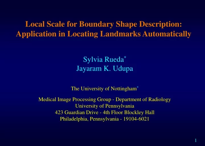
Local Scale for Boundary Shape Description: Application in Locating Landmarks Automatically Sylvia Rueda* Jayaram K. Udupa The University of Nottingham* Medical Image Processing Group - Department of Radiology University of Pennsylvania 423 Guardian Drive - 4th Floor Blockley Hall Philadelphia, Pennsylvania - 19104-6021
Goal Overall:To automatically construct statistical shape models. (Shape models facilitate automatic object recognition, delineation, shape analysis, etc.) Specific: (1) To automatically identify shape-salient points in digital boundaries. (2) To study how effective these points may be for use as landmarks in shape models. (3) To develop algorithms for automatically constructing shape models by using these points.
Why Study Landmarks and Their Automatic Tagging? • Manual tagging is time consuming, tedious, error prone, impossible in 3D, and limits the number of training data sets. • Some landmarks may be more effective than others in capturing shape information. • Landmarks may be useful in studying shape variations – age-based, gender-based, disease-based studies, etc.
Shape Representation vs. Characterization Representation: Methods of approximating and representing shape in the computer. Characterization: Methods of describing the shape as a set of features that result in a minimal representation
Shape Representation (2D) L. da Fontoura Costa and R.M. Cesar, Jr.: Shape Analysis and Classification: Theory and Practice, CRC Press, 2001.
Shape Characterization Boundary-based Shape signatures, moments, polygonal decomp, curve decomp, syntactic, scale space, Fourier descriptors, wavelet descriptors, boundary primitives. Region-based Shape signatures, medial axis transform, moments, generic Fourier descriptors, grid methods, shape matrix, convex hull, primitive shapes. D. Zhang and G. Lu: “A Review of Shape Representation and Description Techniques,” Pattern Recognition, 37:1-19, 2004.
Curvature • A measure of curvature forms the basis of all methods of shape characterization. • (Attneve 1954) • Most methods deal with it directly, others indirectly. • Curvature at a point is the inverse of the radius of the osculating circle at that point. F. Attneve, Some psychological aspects of visual perception, Psychol. Rev. vol.61, 183-193, 1954.
Challenges • How to handle digitization effects and noise in the • boundary? • If a continuous approximation is done first, may • affect shape itself…how much to approximate? • Is it possible to directly work on the digital boundary • and still arrive at shape description?
Scale in Image Processing Scalerepresentslevel of detailof object information in scenes. Scale is needed to handle variable object size in different parts of the scene. Global scale:Process the scene at each of various fixed scales and then combine the results – scale space approach. Local scale: At each voxel, define largest homogeneous region, and treat these as fundamental units in the scene. Lindeberg, T.: Scale-Space Theory in Computer Vision, Kluwer Academic Publishers: Delhi, 1993.
Local Scale At any voxel v in a scene, b-scale:largest homogeneous ball centered at v. t-scale:largest homogeneous ellipsoid centered at v. g-scale:largest connected homogeneous region containing v. Saha P.K. et al. Computer Vision and Image Understanding, 77(2):145-174, 2000. Saha P.K., SPIE: Medical Imaging, 5032:743-753, 2003. Madabhushi A. et al. Computer Vision and Image Understanding, 101(2):100-121, 2006.
Local Scale brain PD slice ball scale tensor scale generalized scale b-, t-, and g-scales can be employed for controlling CAVA processing parameters locally adaptively for better results.
Local Boundary Scale Would like to: • directly work on digital boundary without first approximating it. • handle digital effects and noise. • obtain as complete a shape description as possible with • different levels of detail.
Local Curvature-Scale Shape representation: As an oriented boundary B – a sequence of boundary elements/ points b1,….,bm. c-Scale segment C(bi) at bi: Largest connected set of points symmetrically situated wrt bi such that the distance d of any of these points from a line connecting the two end points of the connected set is within a fixed value t.
Local c-Scale c-Scale value Ch(bi): Chord length corresponding to C(bi) – length of the straight line segment connecting end points of C(bi).
Local c-Scale – Ch(b) Length of object 130, t = 0.02. Ch(b) large small curvature at b. Ch(b) small high curvature at b.
c-Scale – Arc Length, Curvature Chord length versus arc length. Peaks in A(b) mid points of flat segments/inflection points. Valleys in A(b) high curvature points/corners.
c-Scale – Arc Length, Curvature Ch(b) A(b)
c-Scale – Orientation Orientation O(b) at any point b is the angle between the tangent to B at b with respect to the tangent at the starting point b0of B. O(b) b b0 We think of the tangent at b to be a line through b parallel to the c-scale chord at b.
c-Scale – Orientation Orientation O(b) and its derivative O(b). Peaks in O(b) convex high curvature points Valleys in O(b) concave high curvature points.
c-Scale – Orientation Depending on the given shape, O(b) may go beyond 360° and below -360 °.
c-Scale Shape Description c-scale computation median filter peak/valley detection landmark tagging A(b) Af (b) P’s B V’s (B) convex/ concave/ flat median filter first derivative Of (b) O(b) O(b) Input: Oriented digital boundary B. Output: Shape descriptor (n landmarks) – a sequence of n quadruples: concave, flat, convex.
c-Scale Shape Description – Median Filtering Object A(b) Af (b) Window width = 5, filtering two times.
c-Scale Shape Description – Peak/Valley Detection erode dilate erode dilate Bottom hat Top hat Af (b) – Open [Af (b)] Af (b) – Close [Af (b)]
c-Scale Shape Description – Peak/Valley Detection Peaks mid points of straight segments/inflection points. Valley high curvature points/corners.
c-Scale Shape Description – Peak/Valley Detection Parameters controlling details t : should be set just above the level of digitization and other noise. p : Peaks above a certain size in Af (b) are detected. v : Valleys above a certain size in Af (b) are detected. t should be fixed in an application domain. p and v are the only variable parameters.
c-Scale Shape Description – Controlling Detail t = 2 small p , v t = 3 large p , v
c-Scale Shape Description – Tagging Landmarks LM1 : Corners -corresponding to valleys in A(b). LM2 : Midpoints -corresponding to peaks in A(b). LM3:: Endpoints of c-scale segments of LM2 or LM1. Any combination of LM1-LM3 can be potentially used as landmarks.
c-Scale Shape Description – Tagging Landmarks Talus midpoints corners
c-Scale Shape Description – Tagging Landmarks Breast midpoints corners
c-Scale Shape Description – Tagging Landmarks Liver corners midpoints
c-Scale Shape Description – Tagging Landmarks Vertebra midpoints corners
c-Scale Shape Description – Tagging Landmarks Calcaneus corners midpoints
c-Scale Shape Description – Tagging Landmarks Building the ASM model: Model is constructed via a set of landmarks – homologous points. The shape of a given boundary x is described by a vector of n landmarks: The mean shape and the allowable variations are determined from a set of N training shapes given for the object of interest:
c-Scale Shape Description – Tagging Landmarks Align the given shapes to yield: The mean shape is Variations in shape are given by the covariance matrix T.F. Cootes, C.J. Taylor, D.H. Cooper, J. Graham, Active shape models - their training and application, Computer Vision and Image Understanding, 61, (1995), 38-59.
where represents model parameters. c-Scale Shape Description – Tagging Landmarks By selecting largest eigen values of M, the model is given by the pair , where is the matrix of eigen vectors associated with the l eigen values of M. A shape instance can be generated by deforming the mean shape by a linear combination of the eigen vectors:
c-Scale Shape Description – Tagging Landmarks Testing how good a model is: • Compactness: Ability to use a minimal set of parameters. • Generalizability: Ability to describe shapes outside • training set. • Specificity: Ability to represent only valid instances of • shape. • Efficacy: Effectiveness in actual application, such as • segmentation M.A.Styner et al., Evaluation of 3D correspondence methods for model building, IPMI 2003, LNCS 2732, 63-75, 2003.
c-Scale Shape Description – Testing Model Models are compared based on compactness factors: (L = largest number of landmarks tested.) Method 1: c-Scale, mid points and corners. Method 2:Manual landmark selection. Data sets :40 MRI foot images, talus bone, boundary B created via Live Wire segmentation. A.X. Falcao et al. User-steered image segmentation paradigms: Live wire and live lane, Graph Mod & Im Pr.,vol. 60, 233-260, 1998.
c-Scale Shape Description – Testing Model Comparison of methods based on , n = 15, l = 1,…15: manual c-scale P&V l (number of eigenvalues selected)
c-Scale Shape Description – Testing Model Comparison of methods based on , for n = 4, 8, 15: manual c-scale P&V (manual) = 0.72 (c-scale) = 0.79 n (number of landmarks selected)
Conclusions • c-Scale handles digital/noise effects naturally in • deriving shape description. • It facilitates automatic landmark selection. • It produces shape models at least as compact as those • created by manual landmark selection. • It can handle different levels of shape detail.
Conclusions • Unlike scale space approaches, it does not find • corners based on explicit curvature estimation. • It simultaneously finds corners and mid points/ • inflection points. Scale space methods do not • (cannot ?) find the latter. B. Zhong, W. Liao, Direct curvature scale space: Theory and corner detection, IEEE Trans PAMI, vol 29, 508-512, 2007. A. Rattarangsi, R.T. Chin, Scale based detection of corners for planar curves, IEEE Trans PAMI, vol.14, 430-449, 1992.
Future Work • Comparison with scale space methods. • Possible exploitation of other info associated with • landmarks ( A(p), O(p), (p) ) in model building • instead of just the coordinates of p. • Using the model to study object shape variations due • to age, disease, treatment. • Extension to 3D.


![Global scale [> 20000 km] Synoptic scale [2000–20000 km] Mesoscale [2-2000 km] Microscale](https://cdn1.slideserve.com/3357411/slide1-dt.jpg)