Download
1 / 37
380 likes | 556 Views
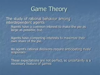
EC930 Theory of Industrial Organisation Game theory -- Appendix. 2013-14, spring term. Review of game theory. Game theory Models rational behaviour when there are strategic interactions between agents

E N D
EC930 Theory ofIndustrial OrganisationGame theory -- Appendix 2013-14, spring term
Review of game theory • Game theory • Models rational behaviour when there are strategic interactions between agents • I.e. when a decision-maker’s payoff depends not only on his/her own actions but also on thoseof other players • Applications • IO: oligopolistic competition, entry deterrence • Bargaining: buyer/seller, employer/worker • Auctions: e.g. 3G licences • Signalling: job market, capital structure • Macro: monetary policy, inflation • Public economics: public good provision, pollution, commons
Elements of a game • Players The agents playing the game • Moves Possible actions that can be taken by the player at a particular node (or stage) • Move order Order in which players can take actions • Information set What is known by a player when s/he moves (prior play, types) • Strategy Complete description of actions to be taken by the player in every contingency • Could include randomisation between actions (mixed strategy) • Payoffs Utility (or profit) to player, as a function of the strategies of all players • Equilibrium concept How to solve the game, to predict play & outcome
Extensive form representation • Tree diagram with nodes and branches, showing • Moves available to each player • Move order • Information sets: single nodes, or 2+ nodes enclosed by dotted line • Payoffs given at terminal node • Notation • Solid node: decision made by a player • Open node: decision made by “nature” • e.g. nature moves to determine a player’s “type” • Dotted lines: indicate player’s information set at that point • i.e. player doesn’t know which node s/he is at
Normal form representation • Matrix diagram • Strategies of 2 players at top & left-hand side • Boxes show payoffs of each player under each strategy combination • Loses the dynamic structure of the game • Normal form game is given by • List of players, i = 1, 2, ..., n • For each player i, a set of strategies Si • For each n-tuple (profile) of strategies (s1, s2, ..., sn), the payoff obtained by each player i
Information conditions • Common knowledge: infinite list of true statements: all players know R, all players know that all players know R, all players know that … • Complete information: the following are all CK • The set of players • Actions available to all players • Potential payoffs to all players • Incomplete information: one or more player lacks some/all of this info
Information conditions • Perfect information: at each node, the player with the move to make knows the full history of play so far • every info set is a singleton (i.e. players always know which node they are at) • Imperfect information: there is at least one non-singleton info set • A game of incomplete info (e.g. uncertain payoff) can be transformed into one of imperfect info (i.e. uncertain type)
A “best response” • Start by defining a best response • Strategy si is a best response for player i to its rivals’ strategies s–i if, s'i(Si), ui (si , s–i) ui (s'i , s–i) • May not be unique (not a strict inequality) • Define rationality • A rational player never plays a strategy that is never a best response (to some set of rival strategies) • Players also take account of the rationality of their rivals, i.e. that rivals do not play strategies that are never a best response
Nash equilibrium (1) • Definition of Nash equilibrium • A strategy profile s = (s1, ..., sn) is a Nash equilibrium if, for every player i = 1, ..., n and s'iSi , ui (si , s–i ) ui (s'i , s–i ) • I.e., the strategy chosen by each player is a best response to those actually played by its rivals • Existence of Nash equilibrium (Nash, 1950) • In an n-player normal-form game, if n is finite and Si has a finite number of elements for every i, then there exists at least one Nash equilibrium (possibly involving mixed strategies) • Proof: uses Kakutani’s fixed point theorem
Nash equilibrium (2) • Alternative way of thinking about Nash equilibrium: consider a player’s incentive to deviate • Does any player have a unilateral incentive to deviate from the proposed equilibrium, given that other players do not deviate? • If not, the strategy profile is a Nash equilibrium • Thus, Nash equilibrium is a stable or self-enforcing concept • C.f. rationalisability • A player’s strategy need only be a best response to some reasonable conjecture about the strategies that rivals will use • Nash equilibrium also requires players’ conjectures to be correct
Example of Nash equilibrium (1) • “Prisoners’ dilemma” • Unique Nash equilibrium: (defect, defect) • The Pareto dominant outcome (collude, collude) does not occur in equilibrium
Mixed Strategy Equilibrium • Example: Matching Pennies Head Tail Head Tail -1, 1 1, -1 There is no sure way to win for either of the players. 1, -1 -1, 1 A reasonable way to play is to randomize between H and T with equal probability. The expected payoff is zero.
Let p, 0<p<1, be player 1’s probability to play H, and q, 0<q<1, be player 2’s prob. to play H. • Player 1’s expected payoff for playing H is: • U1 = -1 . q + 1 . (1-q). • Player 1’s payoff for T is U1 = 1 . q - 1 . (1-q). U1 Player 2 mixes between T and H, she randomizes and plays T with prob. q. 1 T 1 q 0 H -1
We can write best response correspondences in terms of mixed strategy: • B1(q) = 1 if q < ½ B2(p) = 1 if p < ½ • B1(q) = [0,1] if q = ½ B2(p) = [0,1] if p = ½ • B1(q) = 0 if q > ½ B2(p) = 0 if p > ½ q 1 ½ B2(p) The unique Nash Equilibrium is (p, q) = (½, ½). B1(q) 0 ½ 1 p
Example of Nash equilibrium (2) • “Battle of the sexes” • 3 Nash equilibria • 2 in pure strategies: (football, football), (opera, opera) • 1 in mixed strategies • Each player randomises such that the other player is indifferent between their own component strategies • Chris: (2/3 football, 1/3 opera); Pat: (1/3 football, 2/3 opera)
Using Nash eqm in dynamic games • Dynamic game is best illustrated using extensive form (game tree) • Can reduce to normal form (matrix) and find NE • But some NE are “more reasonable” than others (Selten, 1965) • Some Nash equilibria involve incredible threats: strategies involving moves that, if facing that choice, a rational player would not in fact wish to play • Need to refine the concept of Nash equilibrium to eliminate such outcomes and give more plausible solutions
Subgame perfect equilibrium (1) • Start by defining a proper subgame: a part of the game tree that • Begins at a decision node x that is a singleton information set • … but which is not the first decision node of the game • Includes all decision and terminal nodes which follow x(i.e. it contains all “successor nodes”) • … but none that does not follow x • And does not chop up any information sets: i.e. the complete history of the game so far must be CK
Subgame perfect equilibrium (2) • Definition: in an n-player extensive form game, a strategy profile s = (s1, ..., sn) is a subgame perfect eqm (SPE) if • It is a Nash equilibrium of the whole game • And the strategies also constitute a Nash equilibrium of every proper subgame • Thus, every SPE is also a Nash equilibrium • But not every Nash equilibrium is subgame perfect • Existence of SPE • Every finite (in no. of stages and no. of feasible actions) extensive-form game of perfect information has a SPE in pure strategies • Moreover, if no player has the same payoffs at any two terminal nodes, then there is a unique SPE
Example of SPE • Entry game • 2 NE: (enter, accom), (stay out, fight) • Latter involves incredible threat and is not a SPE • Only (enter, accom) is SPE
Repeated games • Special case of dynamic games in which players face same “stage game” or constituent game in every period • overall payoff is a weighted sum or average of payoffs in each stage • past play cannot influence the actions available to players or their payoff functions (since the stage game is identical) • thus, no investments / strategic commitments that alter the rules of the game, nor learning about the environment
Repeated games • But: history of the game does change (as we move through the game-tree), as can players’ one-shot actions • players’ strategies can be conditioned on the earlier actions taken by their opponents new equilibria are possible • in games with imperfect info, the info structure may change over time as private information may be revealed by players’ actions
Repeated games (2) • Examples • Repeated prisoners’ dilemma (collusion game) • Sequential entry game (chain store paradox) • May be finitely or infinitely repeated • If game is finite (in no. of stages and actions), with perfect information, then it has at least one SPE in pure strategies • If the stage game has a unique NE, then the finitely repeated game has a unique SPE in which the NE is played in every round • If stage game has multiple NE, then the finitely repeated game has multiple SPE, and these may include outcomes that are not a NE of the stage game (especially in early rounds)
Infinitely repeated games • Problem • No “last round” so cannot use backward induction • Game is not finite, so existence and uniqueness of SPE cannot be guaranteed • “Folk theorem”: multiple equilibria and indeterminacy • E.g. repeated prisoners’ dilemma • Finite: defect in every round • Infinite: many possible equilibria • E.g. trigger (“grim”) strategy: play C in first round, and continue until rival defects, then play D in every round thereafter • Trigger is a NE of infinitely repeated game, as long as discounting not too severe, in which case outcome is (C, C) in every round
Incomplete information: Bayesian games • In many models, some piece of information is incomplete: unknown to one or both players • Cournot with incomplete info on rival’s cost/type • Entry with incomplete info about incumbent’s cost/type • Auctions: valuations of other bidders • Informationally-challenged player has some prior probability distribution over values/types • In a dynamic game, subsequent events cause this distribution to be updated • How can the game be solved?
Static games of incomplete information • Normal-form representation specifies • Players i = 1, …, n • Players’ action spaces A1, …, An • Type spaces T1, …, Tn (ti is private info to i ) • Beliefs p1, …, pn , where pi (t–i |ti ) • Payoff functions u1, …, un • Timing of a static Bayesian game (imperfect info) • Nature draws players’ types • Own type ti revealed to each player i • Players simultaneously choose actions (aiAi) • Payoffs ui(a1, …, an; ti ) are received
Bayes’ rule • Method for updating probabilities in light of new information (e.g. types of other players, given own type) • Two possible events: A or not A B or not B • We know that Prob(AB) = Prob(A|B) Prob(B) = Prob(B|A) Prob(A) • Rearrange: Prob(A|B) = • Substituting for Prob(B) (as this may occur either with or without A occurring):
Example of Bayes’ rule • Ex ante probabilities, before either player knows own type • Define event A = player A is of type 1 event B = player B is of type 1 • Simple version of Bayes’ rule: Prob(A|B) = • Suppose B knows is of type 1 (i.e. event B has occurred) • Then probability that A is of type 1, Prob(A|B), is given by
Strategies in Bayesian games • A (pure) strategy si (ti ) for player i specifies an action ai for each of i ’s possible types ti • Pooling strategy: all types choose the same action • Separating strategy: each type chooses a different action • Important to specify the action taken by each type because, although the player knows its own type, other players do not know this and will be affected by what they think the player will do
Bayesian Nash equilibrium • Equilibrium concept used in static Bayesian games • Strategy profile s = (s1, …, sn) forms a BNE if • for each player i • and for each of i ’s types ti si (ti) solves • I.e. no player wishes to change its strategy, given the possible types of other players and the actions specified by their strategies • Existence: a finite static Bayesian game has at least one BNE, perhaps in mixed strategies
Example of Bayesian Nash Equilibrium • Cournot duopoly with incomplete info • Profit function ui = qi (i – qi – qj), where i = ai – ci • 1 = 1 (CK); 2 is private information • 1 believes 2 is either high cost (2 = ¾) or low cost (2 = 5/4), each with prob 0.5 • 2’s reaction function given 2: q2(2) = ½(2–q1) [2 eqns] • Denote output choices of high and low types as q2H and q2L • 1 chooses q1 to maximise expected profit given 2’s RF and beliefs about 2’s type: ½q1(1–q1– q2H) + ½q1(1–q1– q2L) • 1’s reaction function: q1 = ¼(2 – q2H – q2L) • Unique equilibrium: q1 = 0.33, q2H= 0.21, q2L= 0.46
Dynamic games of incomplete information • E.g. entry game where entrant is uncertain of incumbent’s cost • Need to combine the earlier concepts • Subgame perfection to eliminate incredible threats • Analyse players’ beliefs to account for incomplete info • Solution concept: perfect Bayesian equilibrium
Example: alternative entry strategies • 2 pure strategy NE: (out, fight), (in1, accom) • First is not reasonable: incredible threat to fight • But only subgame is game as a whole: both NE are subgame perfect
Perfect Bayesian equilibrium (1) • Some definitions • System of beliefs • For each information set, for the player with the move at that set, a system of beliefs specifies a (non-negative) probability (x) of being at each of the decision nodes x in that set • Conditional on having reached that info set • Must sum to 1 • Sequential rationality • A strategy profile is sequentially rational, given a system of beliefs , if the player with the move at each info set does not wish to revise its strategy, given its beliefs about play so far and its rivals’ strategies
Perfect Bayesian equilibrium (2) • Basic idea: at any point in the game, a player’s strategy must prescribe optimal actions from that point on, given • opponents’ strategies (which may include different types) • own beliefs about what has happened so far in the game • beliefs must be consistent with the strategies being played • A strategy profile sand system of beliefs is a PBE if • Strategy profile s is sequentially rational given belief system • Belief system is derived from strategy profile s using Bayes’ rule wherever possible (for info sets reached with positive probability) • At information sets off the equilibrium path, beliefs are determined by Bayes’ rule and the players’ equilibrium strategies where possible (a weak PBE in every subgame)
PBE in entry example • Following entry, accom is the incumbent’s optimal choice for any set of beliefs • Thus (out, fight) cannot be a PBE • (in1, accom) is a weak PBE: incumbent assigns prob = 1 to being at the left node in the information set
Summary of solution concepts • Static, complete info Nash equilibrium • Dynamic, complete info Subgame perfect eqm • Static, incomplete info Bayesian Nash eqm • Dynamic, incomplete info Perfect Bayesian eqm • Further refinements are possible • Forward induction • Trembling hand • Pareto dominant • Markovian